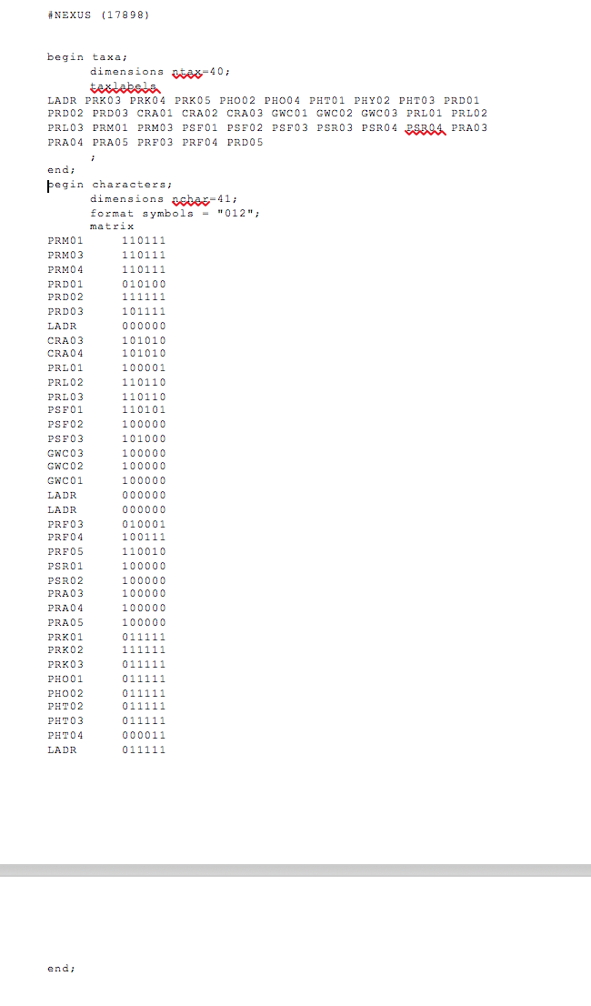
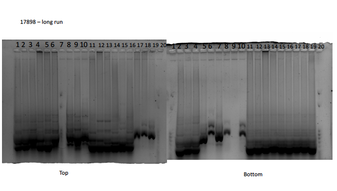
We scored our ISSR gels for two molecular markers: Omar and 17898, on an excel spreadsheet. If there is a band present, we marked it with an 1, if not it’s marked with a 0. I used the short run for Omar and the long run for 17989 because they looked like the bands were easier to see. Then we converted this into a Nexus file. The photos are attached at the bottom!

In lab, we did two Geneious tutorials. One was for a Map-to-reference, and the other was for a De-novo assembly.

Map to Reference tutorial

For the map-to-reference, we learned how to sequence map and SNP calling. We prepared the data by trimming their ends, assembled them, exploring the contigs, how to find SNPs and how to compare them. 5 reads had their ends trimmed due to low quality, they were  55687/1, 135904/1, 96204/1, 145868/1 and 76618/2. It took about 5-10s for the reads to map to the reference genome. There was least coverage at the ends with an average of 98% being covered and the max being  139. When I changed from the highest quality settings to 100% identical, from afar, it looked like there wasn’t any change but if you looked closely, there were a few sites that changed (e.g. site 28, 38, 41 and 73), which shows that there could’ve been a polymorphic site there. The end regions had >2 stdev below the means and we want to exclude them because I assume it’s not reliable? There were some transition sites (site 1554 and 1935), and transversions sites (site 1557 and 1923). I’m not sure if they affected the protein or not. 4 SNPs were excluded from the region. Below is my sequence view of my annotated reference genome with SNP calls along with my polymorphism table (well a chunk of it, it’s a huge file I can’t fit it all in).

De Novo Assembly

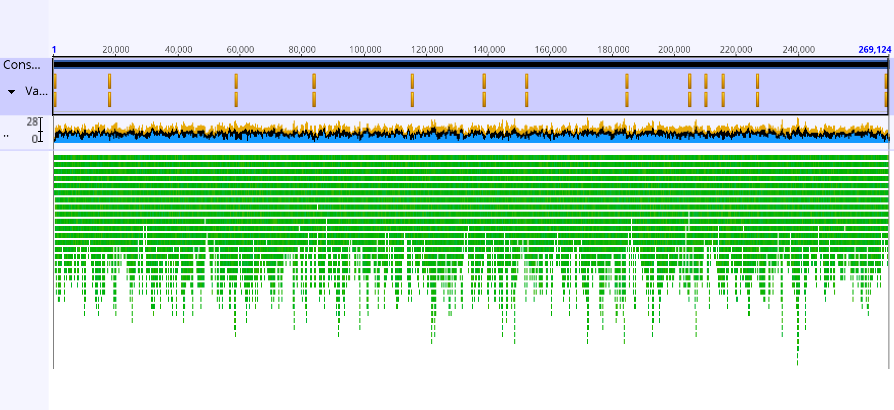
We assembled a bacterial gene in a 3 step tutorial. We assembled the short reads data then we assembled the reads using paired-end information and then we looked at the consensus sequence and tried to fix it. We assembled 2 reads and got back 4 contigs. The mean length of contigs >1000bp is about 130k bp, the shortest contig was around 512 bp. the NC50 score was 192, 891. The De Novo assembly, with and without paired ends, took roughly a minute to complete. There are some sites (15903, 284467) that had no coverage. The final length of the consensus sequence is 269,124bp. The consensus sequence is below.

From all the previous labs, we now have 41 lupine samples from 13 different geographic regions (photo below).

We created a consensus sequence using forward and reverse reads using a program called Geneious. To do so, we select both the forward and reserve reads and did a “De novo assemble” and edited the sequences and extracted the consensus sequences. We did this for all 41 lupine samples. We then ALL of the consensus sequences and used a MrBayes analysis to create a phylogenetic tree with a minimum of 1.5m generations, minimum burn in of 100,000, frequency of 500 and using Lcham as an outgroup and HKY85 as the substitution model.

My tree had a huge polytomy and two clades, with one support value of >0.85. Two of them were from the same georaphic range, and two were not.

We ran our PCR results of the ISSR from last week using a gel electrophoresis to determine which primers worked the best. Not surprisingly, ours didn’t work and the best two primers were Omar and 17898. We used our own original samples from the first time (mine was PSF01-05). And we basically did the same thing as last week: Create 2 mastermixes, one for Omar, and the other for 17898. We got our two strips of tubes of 5), pipetted 1 microlitre of our samples into each tube and add in 19 microlitre of the MasterMix to each respective tubes and ran a PCR.

We received 5 new samples – I got GWC04, PRD04, PRM04, PSR04 and PHO04 and used two molecular markers – ISSR and psbA (since ours failed last week). For the ISSR, we tested out one of four primers (HB10, 17898, Omar, and 844).

The methods for preparing the template DNA is the same (https://usfblogs.usfca.edu/changmargarette/2017/10/23/plant-dna-pcr/)

To create the MasterMix of the ISSR, pipette into a centrifuge tube:

• 12.5 microlitres distilled water
• 3 microlitres buffer
• 1 microlitres BSA
• 2 microlitres dNTP
• 0.25 microlitres primer – 844.
• 0.25 microlitres Taq.

To create the MasterMix of psbA: (https://usfblogs.usfca.edu/changmargarette/2017/10/23/plant-dna-pcr/)

Pipette the 19 microlitres of the mastermix into each respective tube.

We set up a PCR reaction using the 5 plant DNAs that we extracted last week. We used two markers for the PCR: the ITS and psbA.

We clearly labelled two strips of 5 PCR tubes (so that’s 10 total, 5 tubes per strip) with our sample ID and the marker. Pipette 1 microlitre of your plant DNA into the respective PCR tubes, close the lid and place it in eyes.

Next, we prepared two MasterMixes (one for ITS and one for psbA). The steps are as followed:

1. Label two 1.5mL centrifuge tube, one as MM psbA, the other as MM ITS.
2. Thaw the reagents
3. Add 15 microlitres distilled water, 2 microliteres buffer, 1 microlitre BSA, 0.2 microlitres dNTPs and F-Primer and R-Primer, 0.04 microlitres Taw and 1 microlitres of ITS.
4. Repeat step 3 but with psbA.

Now that the MasterMixes have been created, pipette 19 microlitres of the MasterMix into the respective samples (if the PCR tube is labelled ITS, pipette ITS. If not, pipette psbA). Close the lid tightly, mix the tube and place it in the PCR machine.

We were given 5 plant samples (I got the one from Presidio) and inserted each sample into a 1.5mL microcentrifuge tube along with 3 sterile steel balls. We then placed those in a rack and attached it to this wooden block and broke down the cell walls using a reciprocating saw for 40s – the final product looked like a green powder. We centrifuged this so that the green powder would collect at the bottom and then we pipetted 430 microlitres of warm grind buffer to each tube. We placed it in a warm water bath for 10 minutes, shaking it in between and then we pipetted 130 microlitres of potassium acetate into the tubes, mixed them up and placed them in an ice bath. We centrifuged it again for another 20 minutes, labelled a new set of microcentrifuge tubes and pipetted the supernatant into the new tubes, each to its labelled tube. We pipetted 1.5x volume (of the supernatant) of the binding buffer, pipetted all of those into labelled Epoch spin column tubes and centrifuged them. We washed the DNA with ethanol, adding about 500 microlitres of 70% Ethanol to the tubes and centrifuged them, twice to be extra clean (be sure to remove the liquid from the bottom!!). We centrifuged it again, with no liquid this time, to remove any leftover ethanol. We removed the top blue part (the collection tubes) and placed them in clearly labelled microcentrifuge tubes, added 100 microlitres of warm sterile water, centrifuged it again for another 2 minutes to get the elute DNA, which is then placed in ice.

Using our fish DNA consensus sequences, along with around 25 other fish species  sequences and an outgroup (I used a hammerhead shark), that has the CO1 gene, we created multiple phylogenies using different statistical methods. We cleaned up the DNA first, making sure that they all start and end at the same point. We tested out different methods: the Bayesian inference (GTR substitution model). We ran this twice, one for a short period and another one for a long period to see the differences that time could give us. We also used the Maximum Likelihood via rapid bootstrap and rapid hill climbing. The methods produced different consensus trees. For the final tree, we used the MrBayes method (HKJ model) for around 1,100,000 base pairs.

To analyze the DNA that we got, we used an app called Geneious. Seeing how only one of my DNAs worked, I was presented with two other DNA samples. We opened our DNA reads on Geneious and combined the reverse and forward sequences using a function called “De Novo assembly” to assemble a sequence. We edited the sequence by erasing any discrepancies or ambiguity. We used this sequence to generate a consensus sequence and BLAST-ed the sequence, which gives us the scientific name of the species. A google search of the scientific name would tell us the simpler name of the species. After this, we built an alignment by taking some hits from the BLAST results and the consensus sequence and did a “multiple align”.

We travelled up north to the southern end of Point Reyes to Leemantour Beach to find the purple variants of the Coastal Lupines. The drive up was really picturesque, as we drove by the ocean and then into a redwood forest (Samuel Taylor State Park). We spotted a deer out in the wild probably out to mate with another deer. When we stepped foot on the beach, we saw humpback whales in the distance feeding on krill and plankton. We noticed that there were a bunch of birds concentrated on where the whales are at because when the whales feed, they might release some fish up for the birds to eat. We also found the purple lupines! What’s pretty epic about them is that the plate that is on the beach was originally where Santa Monica is so it’s like a whole new different population! I’m curious now to find if the genes for this lupines and the lupines down south in SoCal are similar. We stopped by Samuel P Taylor State Park to find another plant, but we couldn’t find them.

The next week, we ran two gel electrophoresis on our fish DNA, one for our gDNA and one for our PCR product. The agarose block was prepared for us already (well for the first one) and all we had to do was pipette our sample into the wells and run the gel electrophoresis for about 10 minutes at 145V. To prepare out samples, we pipetted 2 microlitres of loading dye on a piece of parafilm and pipetted 3 microlitres of our DNA onto it. We repeated this step for our PCR product BUT we reused our old agarose gel by melting it and letting it cool and set. After determining which PCR worked, we did an Exosap PCR Clean up. We first made a master mix per table consisting of water, buffer, Exo and SAP, and then we pipetted our PCR product into a PCR tube and pipetted 12.5 microlitres of our master mix in the tube. After this, we put the tubes in a thermocycler and ran the program and after it’s done, we put it in the freezer.

For my gel electrophoresis, only 2/3 of my fish samples worked. This is probably because I only realized till the end of the first lab that I was using the pipette wrong so I probably have the wrong volumes used.