Today we followed two tutorials to learn how to assemble genomes. For one, we mapped against a reference genome. For the other, we assembled the genome de novo, meaning we had no reference.
Today we followed two tutorials to learn how to assemble genomes. For one, we mapped against a reference genome. For the other, we assembled the genome de novo, meaning we had no reference.
Lupine ISSR Gel
Today, we ran out our ISSR PCR reactions on one large gel. The gel is 2% agarose, denser than normal to allow better separation of bands.
Steps for loading the gel were simple and as follows.
I loaded my samples and Danielle’s samples. I also accidentally added one of Daniel’s samples twice; I believe it was sample 4 but it may have been 3-7.
Prof Paul imaged the gel after class.
New Mimulus alignment and concatenation
During lab we also created another alignment of our Mimulus cardinalis sequences. Prof Paul was able to get sequences for several new populations, so we edited the sequences for our given EPIC marker and then included them with the sequences we worked with a couple weeks ago create an alignment with all of them.
We then uploaded our alignments onto Canvas so that we could use other people’s alignments with other EPIC markers. I downloaded Nathalia’s 5525 alignment, Prof Paul’s 5534 alignment, and Jinwoo’s 5551 alignment. I then concatenated all of the alignments to create one set of sequences to build a tree out of.
Today we performed PCR using ISSR primers on previously extracted Lupinus arboreus samples. ISSR stands for interspersed simple sequence repeats, which are microsatellites. Instead of using the microsatellites as the markers, we use them as primers to generate fragments of DNA through PCR. We will then compare the length of these fragments to better understand population genetics of Lupinus arboreus.
Dilution
First we each received 5 samples. Then, for each sample, we made three 1:10 dilutions so that each table could work with each sample. Additionally, PCR for these ISSR primers works better with diluted gDNA.
My samples and ISSR primer
Every table worked with the same 60 samples, but each table used a different ISSR primer. My table worked with the primer HB10. I also included a negative control. Below is table showing my samples and their corresponding label on their PCR tube. I also labeled each strip with my intials, AJC, and HB10.
| Label | Sample ID |
| 1 | PSF01 |
| 2 | PSF02 |
| 3 | PSF03 |
| 4 | PSF04 |
| 5 | PSF05 |
| 6 | CRA01 |
| 7 | CRA02 |
| 8 | CRA03 |
| 9 | CRA04 |
| 10 | CRA05 |
| 11 | PRA01 |
| 12 | PRA02 |
| 13 | PRA03 |
| 14 | PRA04 |
| 15 | PRA05 |
| 16 | Negative control |
Master Mix
Vanessa prepped the master mix as shown below, working on ice. Except Prof Paul added the taq at the end just before we add the master mix to our PCR tubes and put them in the thermocycler. Vanessa made enough Master Mix for 80 samples (our table had 64 total)
| Material | per rxn (µL) | per 80 rxns (µL) |
| pure H2O | 12.5 | 1000 |
| 10x buffer + Mg | 3.00 | 240 |
| BSA | 1.00 | 80 |
| dNTPs | 2.00 | 160 |
| HB10 primer | 0.25 | 20 |
| Taq | 0.25 | 20 |
PCR prep
We first prepped our PCR tubes by adding 1 µL gDNA to each appropriately labeled tube. Then we added 19 µL of master mix to each tube. I pipetted up and down to mix each tube. Samples were kept on ice until they were placed in the PCR machine and ran.
Today we edited and aligned Mimulus cardinalis sequences in Geneious. Since our PCR attempts did not work, we worked with an older dataset. I worked with sequences from the 5536 EPIC marker.
1. First alignment
I did a muscle alignment of the sequences to do a first round of editing. First, I trimmed the ends to remove areas of poor quality. Next, I looked for polymorphisms and heterozygotes. There were about 10 polymorphic columns, and 3 heterozygote columns. Some sequences were not read as heterozygotes despite having two peaks, so I looked through the columns to edit any obvious heterozygotes with the correct code. Lastly, I edited any areas of obviously poor quality within the sequence. I then saved the alignment and edits to the sequences
2. Assemble forward and reverse reads and generate consensus sequences
I assembled each pair of forward and reverse reads. I then checked the assembly again for any area of poor quality or heterozygotes that I missed on the last step. I did not need to edit much since I edited on the previous step. Almost all of each assembly was of very high quality. I then generated the consensus sequences for all of the pairs. I then edited the names so that they were just the sample ID, so that they can be aligned with the same samples for the other EPIC markers. Two samples, JP1167 and the outlier M. lewisii sample, only had one read so I did not generate consensus sequences, but checked them for any necessary edits and used them in the alignment in the next step.
3. Final alignment
Using the consensus sequences, I built a MUSCLE alignment again. I looked at the alignment to see if any edits were again necessary, but I did not make any.
4. Infer Bayesian tree
At home, I ran a bayesian analysis to infer a tree. I used TG0248 (M. lewisii) as the outgroup, and ran it with a chain length of 3,000,000, a burn-in length of 300,000, and a subsampling frequency of 500. My tree had no strongly supported clades and was one giant polytomy.


Today we ran gels for our DNA extractions from last week and then set up and ran PCR.
As usual, the gels were already set up, so we mixed our extractions with loading dye on parafilm, then loaded the gel. We ran the gel at 140V for 20min, then imaged it (see below). All extractions were successful for the possums.
Next, we aliquoted 20 µL of each of our extractions into two more tubes to share with the other tables. Each table worked with a specific EPIC marker for all samples, so each table needed DNA extraction from each sample. We did however remove two samples in which the extraction did not work and two from a population that was overrepresented, so we were working with a total of 32 samples. The 32 samples were split among the 4 people at each table, so each person worked with 8 samples.
The three EPIC markers were 5334, 5525, and 5536. My table worked with 5536.
The samples that I prepped for PCR were:
| Tube Label | Specimen ID |
| 1 AC | JP 1229 |
| 2 AC | JP 1299 |
| 3 AC | JP 1302 |
| 4 AC | JP 1309 |
| 5 AC | JP 1311 |
| 6 AC | JP 1315 |
| 7 AC | JP 1316 |
| 8 AC | JP 1322A |
We did the following steps to prep for PCR:
| Material | per rxn (µL) | per 40 rxn (µL) |
| ddH2O | 15.0 | 600 |
| 10x buffer + Mg | 2.00 | 80 |
| BSA | 1.00 | 40 |
| dNTPs | .20 | 8 |
| F-primer 5536 | .20 | 8 |
| R-primer 5536 | .20 | 8 |
| Taq | .04 | 1.6 |
We extracted DNA from samples of Mimulus cardinalis and Mimulus guttatus. Most samples were from M. cardinalis centered around collections from Mt. Tam, but also including collections from Mt. Diablo, Big Sur, and near Mono Lake.
My samples were JP1308 (M. cardinalis), and JP1316 and JP1320 (both M. guttatus from Mill Creek near Mono Lake).
We used a modified Alexander et al protocol. Steps are as follows, including notes and details about my extraction today:
This week we built a phylogeny using our fish samples and COI sequences from NCBI downloaded through geneious.
ALIGNMENT
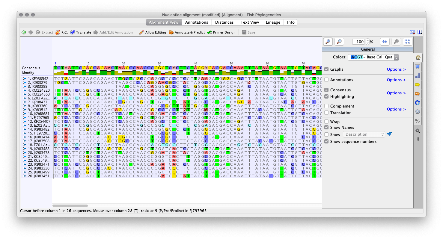
First we created an alignment of all of our sequences, then edited it so that we had trimmed edges, similar to last week. Additionally, we looked to see if any sequences lined up especially poorly. This may happen because the sequence is a reverse read relative to the others. Two of my sequences lined up especially poorly, so I reveresed them. They still lined up poorly, so I removed them and redid the alignment. Below is an image of the alignment after editing:
MODEL of MOLECULAR EVOLUTION
Next, we inputted our alignment into the program jModelTest2 to find the best model of molecular evolution. We exported the alignment as a phylip file and computed likelihood scores. We then used the program to calculate Aikake Information Criterion and Bayesian Information Criterion scores. The lower the AIC or BIC score, the better the fit. For both AIC and BIC, the model TPM2uf+I+G scored the lowest. This model was ranked 40, so it was moderately complex.
MrBayes
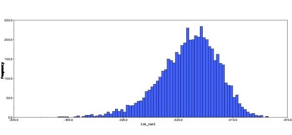
We used the MrBayes plugin in Geneious to build our first tree. First, I chose a subsitution model. Since TPM2uf was not available, I chose HKY85, which is similarly complex. For the rate variation, I chose invgamma because my model above had “+I+G” in it.
I ran a short analysis to test the waters, with a chain length of only 10,100 and a burn in of 100. The tree produces had many polytomies, branches with low probabilities, and the density and trace plots showed signs of not running the analysis long enough. I then ran the analysis again with a chain length of 110,000 and burn in of 10,000. This tree had fewer polytomies and greater probabilities. The clades were similar, but not the same. Lastly, the density plot showed a better distribution of probabilities and the trace plot looked like a fuzzy caterpillar. After class, I ran the analysis at 3,000,000 with a burn-in of 300,000. This produced a tree with even fewer polytomies and better probabilites.
RAxML
Next I used the RAxML plugin to build a maximum likelihood tree. We used rapid bootstrapping with rapid hill climbing with a bootstrapping parameter of 100. This created a file with 100 trees, so I created a consensus tree of those. This tree had many, many polytomies but the clades with high support did match clades in the MrBayes analysis.
PHYML
Now I used PHYML to build another maximum likelihood tree. Again we used 100 bootstraps. This tree produced many fewer polytomies than RAxML. Many clades had agreement with the MrBayes trees, but there were a several taxa placed in pretty different parts of the tree.
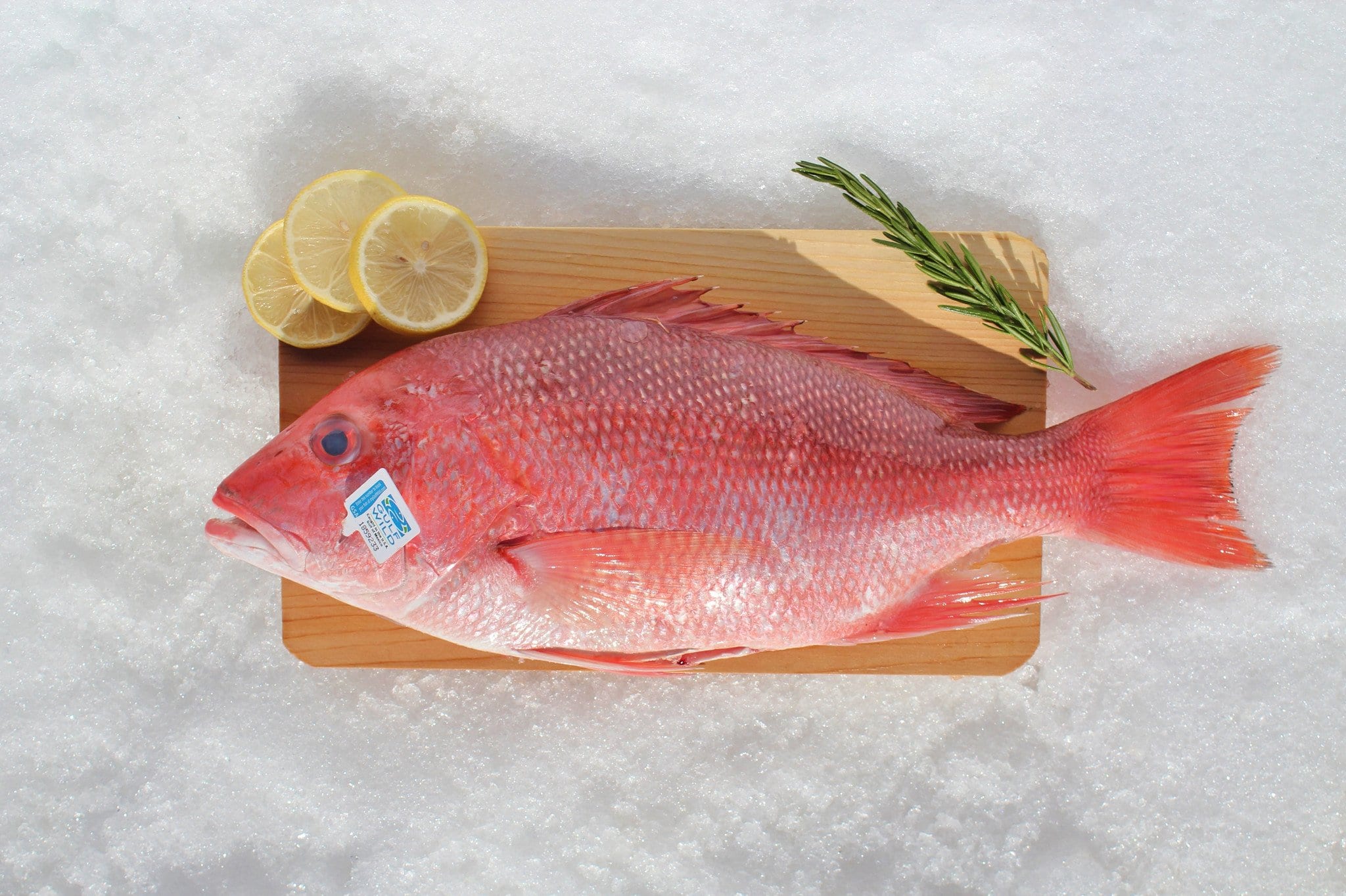
Neither of my two samples that were sent for sequencing worked, so I worked with three of Elaine’s samples. They were labeled as white tuna, red snapper, and yellowtail.
First, we loaded the sequences into Geneious, and spent some time becoming familiar with the layout of the program, how to read the sequences, and how to edit them.
Each sample has a forward read and a reverse read. We assembled the two together, which allows us to see what the consensus sequence looks like. The sequence reads can be of varying quality, so creating a consensus of the forward and reverse read gives a sequence we can have greater confidence in. Some parts of each read may be of low quality, so if the other read was high quality in that area then we have a good idea of what those bases should be and the consensus should reflect that. Below is an image of the program while viewing the De Novo assembly.
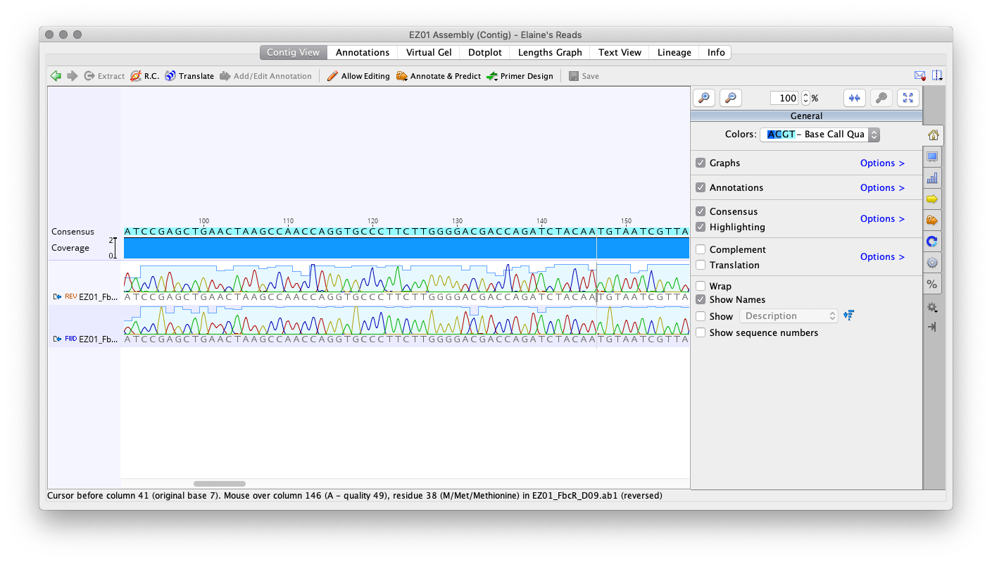
Now we need to edit the reads to make sure the consensus sequence that we generate reflects the areas of high quality in our reads. The beginning of each read is usually of low quality, so we trim those areas down. Additionally, we had to look through the rest of the sequence to spot bases labeled with “N”. This may be due to the two reads conflicting, but one read may have a much higher quality read than the other. So we should edit the poor quality read to match the other. Elaine’s samples had no low quality reads within the sequence, so I only had to trim the ends. Once finished editing, we created the consensus sequence.
We used BLAST (Basic Local Alignment Search Tool) to compare our consensus sequence to a database of other sequences. Elaine’s reads were all of great quality, so the top hit’s for all three samples ranged from 99.8%-100%.
BLAST Results:
Labeled White Tuna – BLAST Thunnus alalunga (Albacore)
Labeled Red Snapper – BLAST Oreochromis niloticus (Nile Tilapia/gross)
 ≠
≠ 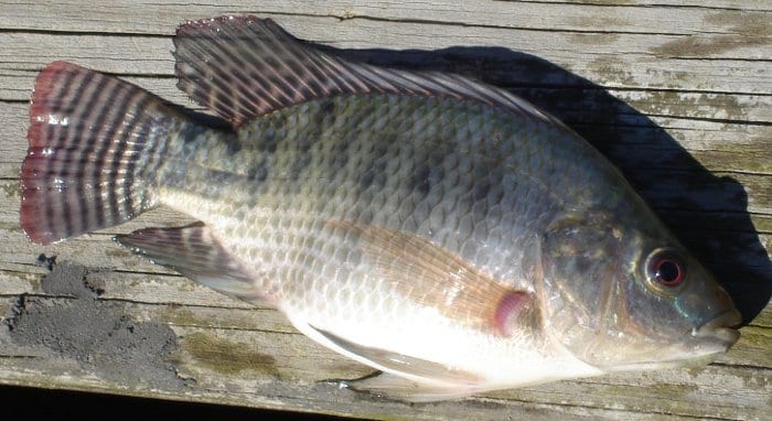
Labeled Yellowtail – BLAST Seriola quinqueradiata (Yellowtail)
Sequence Alignment with top hits:
Next and last, I aligned the white tuna sample sequence with 5 other Thunnus alalunga sequences from the BLAST search. Across the 5 sequences, there were only two polymorphism, at site 443 and 530. At both sites, the polymorphism was between 2 bases, C and T.
Today we drove north of the city, in search of Mimulus cardinalis and purple-flowered Lupinus arboreus. We drove from the east side of Mt. Tam to the west side.
On the east side, we first stopped at Alpine Dam and hiked down to Lagunitas Creek, typical habitat for Mimulus cardinalis. Although we didn’t find any individuals there, we had an adventure getting down and saw a congregation of ladybugs. This side of the mountain is much drier, but Mimulus cardinalis occurs in wet areas like the creek. We stopped another time on this side of the mountain, at a seep in the side of the road. There were a couple individuals, without flowers, that were nearing the end of their lives. Although their habitat is quite different from the lupines from last week, they have a similar patchy distribution. On Mt. Tam, they are often in small populations in wet habitat like this.

We then drove over Mt. Tam and west towards the coast. Fog was coming in and the ocean was hardly visible. Eventually, we were driving among a coastal scrub community similar to what we saw last week. We stopped at a pullout and saw some of the plants as last week: coyote brush and bush lupines. Lupines here had purple flowers. The individuals were scattered sparsely around the area in the same manner as last week.

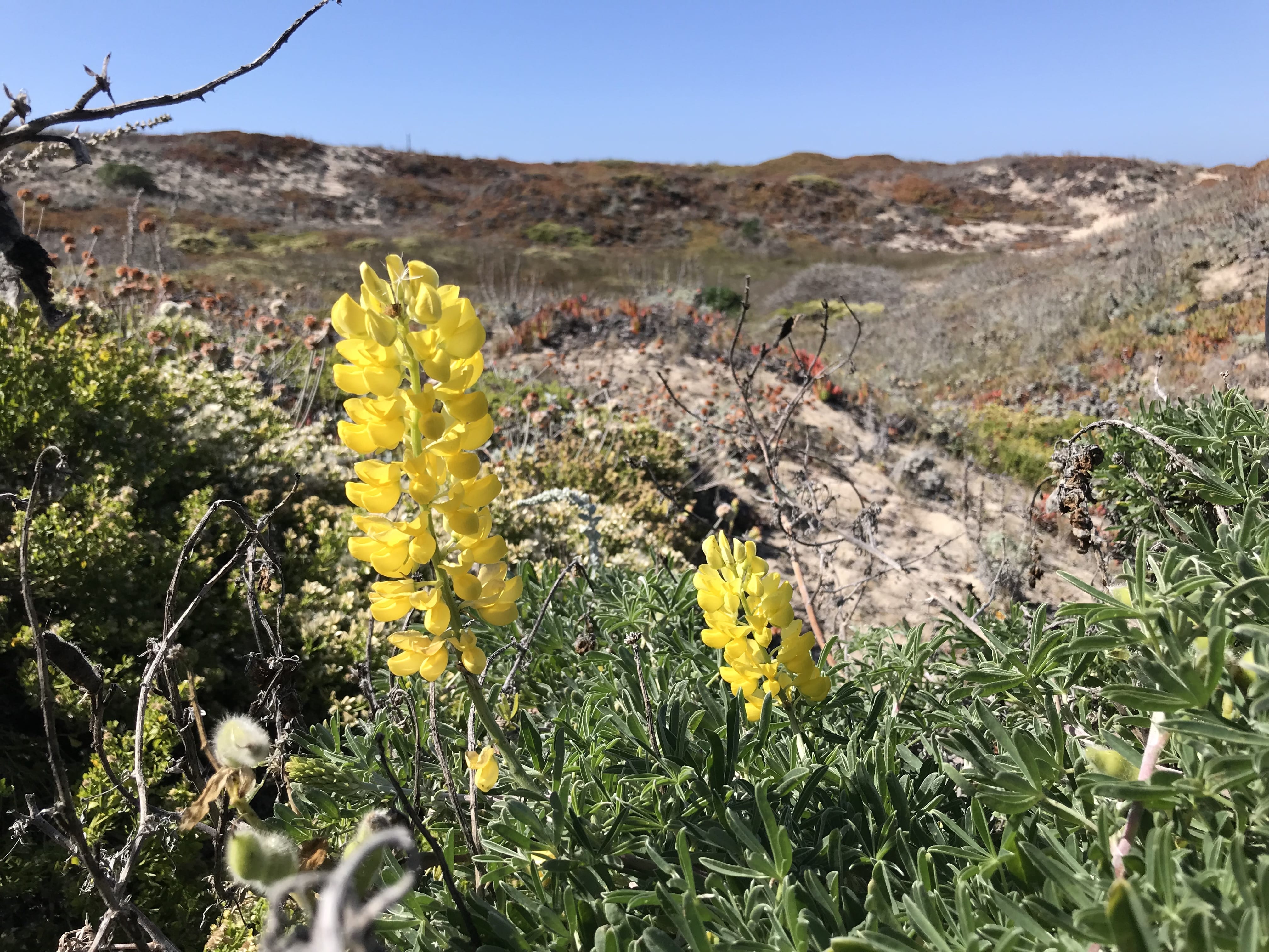
We drove south to Pescadero Beach in search of flowering Lupinus arboreus. We first walked around the coastal scrub community on the bluffs behind the shore. We spotted some lupines, but none flowering. In the coastal scrub community, coyote brush and coast buckwheat were very common, along with the invasive ice plant.
We discussed the stresses faced by coastal plants: salt spray, sandy soils, high winds, and high sun exposure. However, being a coastal plant has its benefits since the proximity to the ocean means there is relatively little daily and seasonal temperature fluctuation.
The bush lupines were few and far between, though they stood out since they appeared to grow taller than other plants in the community. We walked down along the beach and behind the dunes in search of a flowering lupine. We found a couple with a few inflorescences still in great shape, though they were mostly in fruit. My hikes along the CA coast have mostly been in Marin Co, so when I thought of bush lupines, I thought purple flowers. It was interesting seeing, or at least paying attention to, these yellow-flowered bush lupines for the first time.