Melissa Hernandez's Molecular Ecology Lab Notebook

In this lab, we began by downloading tutorials for reference-based assembly and for de novo assembly. Once downloaded, files were imported into Geneious.

The reference-based assembly worked with a dataset of Illumina sequence reads that map to a single gene in the E. coli genome. The first step was trimming the data according to the default settings. Next, trimmed reads and the reference sequence (yghJ CDS) were assembled via mapping to reference. Following the assembly, a contig of the reads mapped to the reference and an assembly report were generated. High and low coverage of the reference sequence and the consensus sequence. The next step was detecting SNPs in the mapped data using the Find Variations/SNPs under the Annotate/Predict menu. An annotation track was added to the reference sequence following this step. Additionally, a table of all the annotations on the sequence was generated, which included polymorphism annotations. Finally, SNPs were filtered based on their overlap with another annotation track or annotation type. Specifically, SNPs that were present in regions of low coverage were filtered out. Below are responses to questions regarding the reference-based assembly tutorial.

1. Five reads that had their ends trimmed due to low quality bases included: #10 (185658/2), #11 (55687/1), #18 (191505/2), #23 (135909), #53 (190007/2).
2. I think paired-end reads are more important to use for de novo assembly because reference-based assembly entails utilizing already sequenced genomes as a reference for mapping the location of reads. In other words, the reads are aligned to the reference sequence. With de novo assembly, there is no prior sequence knowledge, thus paired-end reads can provide information about the sequence on each end.
3. It was a relatively quick process for the reads to map to the reference genome. According to the yghJ paired Illumina reads assembled to yghJ CDS (divergence reference) Report, it took about 7.02 seconds.
4. When the yghJ CDS (divergent reference) sequence was assembled to the yghJ paired Illumina reads, 5,058 of 5,060 reads were assembled. In addition, there was a coverage of about 4, 581 bases, with an average coverage of about 98.1 bases. This assembly yielded a maximum coverage of about 139 and a minimum of 1. The following intervals of the assembly contained the lowest coverage: 1 – 43, 121 – 173, 294 – 310, 4303, 4338 – 4401, 4435, 4499 – 4581. These intervals were located either at the beginning or at the end of the consensus sequence. Thus, they might have been insufficient reads to accurately identify the bases at these ends.
5. When the consensus sequence changed between using a “100% Identical” and “Highest Quality” consensus, the four following sites changed: #20 (R à A), #38 (M à C), #84 (W à T), #127 (R à G). In terms of polymorphism, these sites reveal that there are two possibilities of bases that can be present in the reads. As a result, this can lead to large variety.
6. One region in the sequence that had >2 standard deviations below that mean in coverage was 4467 – 4483. We would not want to classify this region as a SNP because there was too much variation in this region. With SNPs, we are only looking for a site where there is a base difference. In this region, however, it is possible an incorrect fragment was added, although there was a single base pair difference.
7. Two CDS positions where there was a transition mutation include CDS position 4,575 (A to G) and CDS position 4,464 (A to G). Two sites where there was a transversion mutation includes CDS position 4,485 (G to T) and CDS position 3, 614 (C to A).   For the latter transversion mutation, there was an effect on the protein. The former transversion mutation had no effect on the protein.
8. Below is a screenshot of the polymorphism table.

9. One region of low coverage that was excluded using the “Compare Annotations” tool in Geneious that did not result in excluding SNPs was region 4,499 – 4,581. In this region, 12 SNPs were not excluded. One region where SNPs were excluded included 4,438 – 4,581.                                                                           10. Below is a screenshot of the annotated reference genome with SNP calls.

 

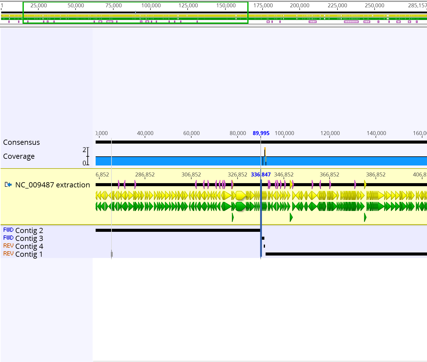
The de novo assembly tutorial utilized short read next-generation sequencing data to perform a de novo assembly of a section of the Staphylococcus aureus genome. First, the reads were assembled using de novo assembly. An assembly with 4 contigs was produced. To see how the contigs align to the original sequence, sequences were assembled using Map to Reference under the Align/Assemble menu. In the region around 90,000, there was no reconstructed contig, which is why the two longest contigs could not be joined. Next, two sets of reads were combined into a single paired reads file. Once the paired reads file was created, De Novo Assemble was selected from the Align/Assemble menu. The resulting consensus sequence was mapped to the NC_009487 reference sequence. A final contig was generated that was almost full in length with a few positions that were ambiguous due to errors in the original data. The bases were corrected using the Find Variants/SNPs under the Annotate and Predict menu. Ambiguous bases in the consensus sequence such as “R” were changed according to a “0% – Majority” threshold. The final step in the tutorial was remapping the new consensus sequence to the NC_009487 sequence.

1. From the assembly, 25, 172 reads were assembled along with 4 contigs that were produced. The largest contig (contig 1) was assembled using 17, 994 reads. The minimum length of the shortest contig (contig 4) that was assembled from 42 reads was 512 bp long. The means of length of contigs >1000bp was 133, 444 bp. Finally, the yhe NC50 score for this assembly was 1.
2. The de novo assembly took about 17.06 seconds, slightly longer than the reference-based assembly. Contig 4 had the lowest maximum coverage and contig 1 had the highest maximum coverage.
3. The region of that had no coverage was 90,759 – 92,269. This region was where the longest contigs could not be joined.
4. The de novo assembly with paired data took about 5.61 seconds; this assembly took less time than the two previous assemblies.
5. Correcting the Paired Reads Assembly sequence was necessary because it contained ambiguous bases. These regions might have been the product of poor assembly or read errors. By correcting the bases in the consensus sequence, we can ensure there is consensus between the sequences and the consensus sequence. Also, it ensures that the consensus sequence contains the most common base relative to the other sequence.
6. The final assembly sequence that was constructed using the pair reads sequence and the NC_009487 extraction sequence was 285,156 bp long. Below is a screenshot of the final consensus sequence that was generated.

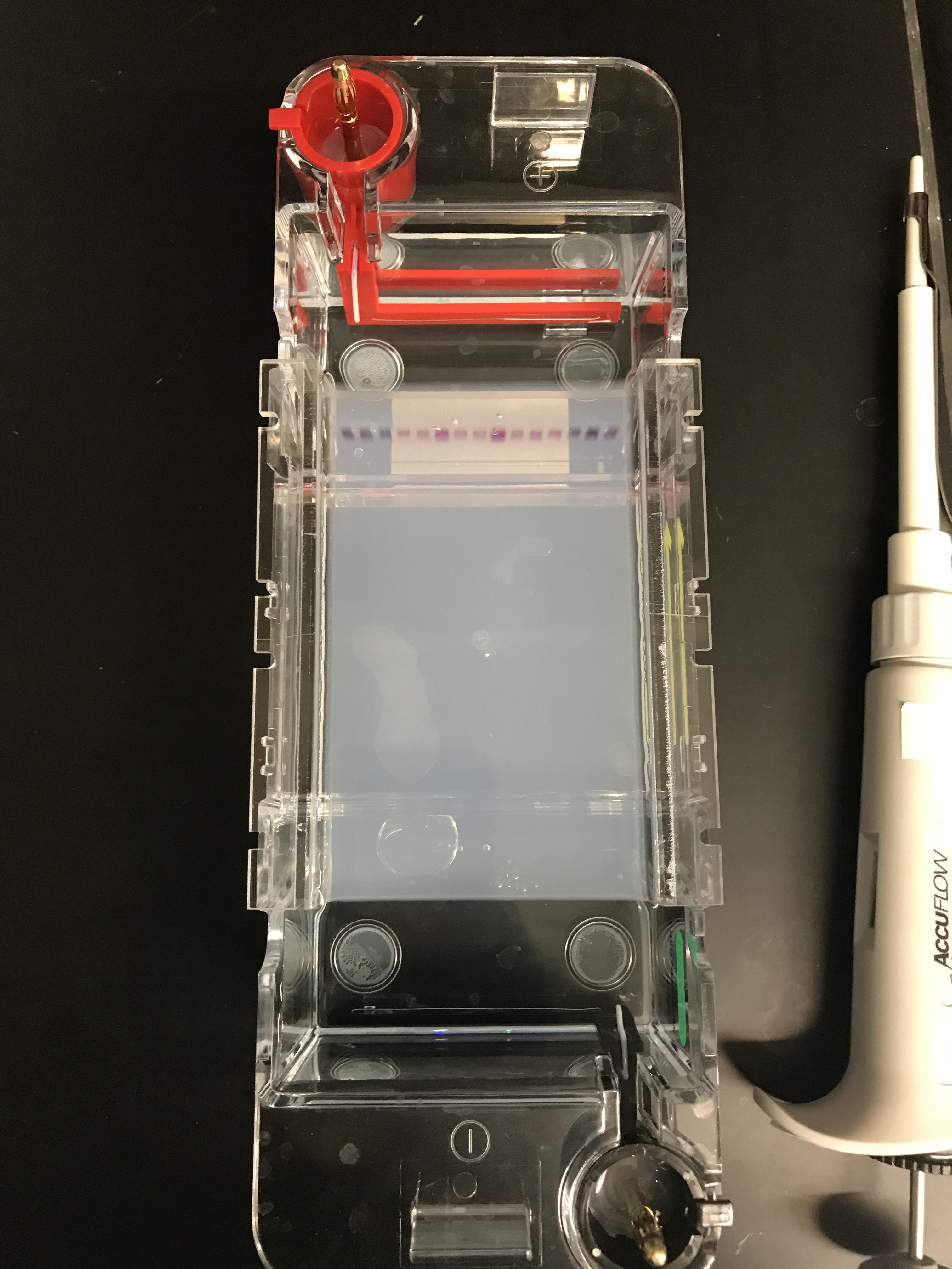
The second part of the lab entailed scoring the ISSR gels for each primer (Omar and 17898) for banding – a “1” if a band was present and a “0” if a band was not present. After the bands were scored, results were transferred into an Excel spreadsheet. Next, a nexus data file was formatted using the “ISSR_data_format_example” as a template. The matrix was pasted into the data file, “taxa labels” were added that corresponded to the names of the individuals, and the nchar was set to 11 to account for the total number of bands scored. Because not all classmates chose the same three individuals to use for both primers, two nexus files were generated, one for each marker. Below is a screenshot of each nexus file.

Nexus file for 17898 primer:

Nexus file for Omar primer:

 

The first part of this lab was performing a gel electrophoresis of our ISSR samples. After obtaining the ISSR strips (17898 and Omar ISSRs were used) assembled last week, three samples from each strip were selected to perform the run. The following samples were selected from strip 1 (17898): PRK01, PRK02, PRK03. From strip 2 (Omar), samples PRK13, PRK14, PRK15 were selected. 1 µl of loading dye was transferred to each of the six samples using a p10.

The samples were loaded into the appropriate ISSR gel tray. The gels ran at 60 volts for 1.5 hours.

Next, an ITS alignment was assembled in Geneious utilizing forward and reverse reads of the ITS marker for 41 individuals of Lupinus arboreus collected from 13 geographic regions.

An assembly was constructed using the forward and reverse sequences for each individual. Once the assembly was complete, the sequences were edited. Unsuccessful regions at the beginning and at the end were trimmed and incorrect base calls and ambiguous bases were amended.   Then, edited consensus sequences were extracted. These steps were repeated for all 41 individuals.

An alignment was assembled using the 41 consensus sequences extracted in the previous step. The alignment was edited by trimming the ends so that sequence lengths were in agreement. The edited ITS alignment was used to construct a phylogenetic tree using the MrBayes tool in Geneious. The MrBayes analysis was run using the following parameters: Chain length was set as 1,500,000; Burn-in Length was set at 100,000; HKY85 was selected as the substitution model; and 500 was set for the Subsampling Frequency.

The following phylogenetic tree with support values was generated.

Below are the posterior distribution and the trace from the MrBayes run.

The tree included one clade with a support value of 0.9895. The individuals of this clade were PRD05, PSF03, GWC01, and GWC02. PRD05 was located at Drakes Beach in Point Reyes, PSF03 was obtained from Presidio, GWC01 and GWC02 were obtained from Grey Whale Cove State Beach.  PRD05 was collected from a mixed lupine plant. PSF03, GWC01, and GWC02 were sampled from a yellow flowered lupine plant.

Based on the individuals represented within each clade of the phylogenetic tree, it can be concluded that the individuals are found in geographically close populations, rather than in the same population. Some individuals with purple flowers were found in the larger clade, where most yellow flowered individuals were grouped. In addition, not all purple flowered individuals were grouped in the same clade. Individuals from purple flowered samples (PHO, PHT, and PRD) were present in the largest clade and in a clade with a support value of 0.9805 or 0.7472.

As previously mentioned, the internal transcribed spacer (ITS) is found in fungi and was utilized as a primer to perform PCR reactions with DNA extracted from the leaflets collected from lupine plants. In assessing the phylogenetic relationships of the Lupinus populations, it appears that ITS does not provide enough resolution to distinguish populations phylogenetically. Some samples of either the purple or yellow flowered individuals were not grouped together in the same clade. If these samples were present together, then ITS could have been successful at the population level.  Finally, the presence of the polytomy indicates phylogenetic uncertainty, in that we cannot determine how the individuals are related.

ISSR amplification reactions made last week using 5 random extracted DNA samples (belonging to other students) with the 17898 ISSR were used for gel electrophoresis. 1 µl of loading dye was added to each PCR reaction tube using a p10. Pipette tips were changed between each sample.

Using a pipette of the same size, 10 µl of each DNA-loading-dye mixture was added to the appropriate well. The gel was run at 60volts for 1.5 hours.

After the run, the gel tray was scanned to determine successful ISSRs.

Successful ISSRs included Omar and 17898.

Next, 1:10 dilutions using our extracted DNA samples (Lab 9) were made. 5 1.5mL centrifuge tubes were labeled with the corresponding sample ID and “1:10.” Labels are as follows: PRK01 1:10; PRK02 1:10; PRK03 1:10; PRK04 1:10; PRK05 1:10.  Using a p10, 10 µl of sample DNA was added to the appropriate centrifuge tube. A p200 was used to add 90 µl of ddH₂O to each tube. Assembling dilutions ensured the concentration of potentially present plant secondary compounds were minute, as these compounds could affect PCR success.

Two 0.2 mL 5-tube strips for suitable for PCR were labeled with the appropriate sample ID (tubes of strip 1 were labeled as follows: PRK01, PRK02, PRK003, PRK04, PRK05 and strip 2 was labeled as PRK11, PRK12, PRK13, PRK14, PRK14, PRK15). Contents in strip 1 were used to perform PCR using 17898 and Omar was assigned to strip 2.

1 µl of 1:10 diluted DNA was added to the corresponding tubes of strips 1 and 2 using a p10. Pipette tips were changed after each sample.

For each ISSR, a master mix was made that included all the reagents necessary to perform the PCR reaction. By creating a master mix, the likelihood of errors associated with pipetting small volumes were minimized. The ingredients and associated volumes used for each PCR reaction are as follows: 12.5 µl ddH₂O; 3.00 µl 10x buffer +Mg; 1.00 µl BSA; 2.00 µl dNTPs; 0.25 µl primer; 0.25 µl Taq. The primer corresponding to each ISSR was added to the appropriate master mix. Volumes were multiplied by 20 to compensate for the quantity of reactions for the group.

A p200 was used to transfer 19 µl of the master mix containing the 17898 ISSR to each tube of strip 1. 19 µl of the master mix containing the Omar ISSR was added to each tube of strip 2. Finally, strips were placed into PCR machine.

 

In this lab, 4 interspersed-simple-sequence-repeat (ISSR) primers were tested via performance of PCR reactions. An ISSR is a dominant marker that utilizes microsatellite repeats (followed by two arbitrary bases) as primers to amplify adjacent potions of the genome. Once amplified, the DNA pieces can be visualized on an agarose gel for length polymorphisms. Although ISSRs do not distinguish homozygotes from heterozygotes, they are useful for intraspecific population level studies.

The following ISSR markers were tested: HB10 – (GA)⁶CC; 17898 – (CA)⁶AC; Omar – (GAG)⁴RC; 844 – (CT)⁸RC. Each lab group was assigned one ISSR mentioned above. Our lab group was assigned 17898 – (CA)⁶AC.

5 random extracted DNA samples belonging to other students were utilized for this PCR reaction. First, 1 0.2 mL 5-tube strip (PCR tubes) was labeled with tube numbers and sample IDs (Tube 1 – PRA02; Tube 2 – PRK02; Tube 3 – GWC02; Tube 4 – CRA04; Tube 5 – PRD05). Using a p10, 1 µl of template DNA was added to the appropriate PCR tube. Pipette tips were changed between samples to prevent contamination. Once PCR tubes were filled with template DNA, they were placed on ice.

A master mix was made with the following reagents and volumes: 12.5 µl ddH₂O; 3.00 µl 10x buffer +Mg; 1.00 µl BSA; 2.00 µl dNTPs; 0.25 µl 17898 primer; 0.25 µl Taq. To each amplification reaction, 19 µl of master mix was added with a p200. PCR tubes were placed into PCR machine.

Next, PCR protocol described in “Lab 10 – Plant DNA PCR I” using a primer for the psbA marker was followed due to unsuccessful results that were obtained. The following samples were used to perform the amplification reaction: PRA02; PRK02; GWC02; CRA04; PRD05. 1 0.2 mL 5-tube strip was labeled with the above sample IDs and tube number. More information regarding the protocol followed and reagents and volumes used can be found here.

 

The first step in this lab was to load gels using DNA extracted from plant samples previous lab. A p10 was used to pipette 5 “dots”of loading dye, each of 1 µl onto Parafilm. Using a pipette of the same size, 3 µl of the template DNA was added to the appropriate loading dye “dot.” Once the extracted DNA was added, a p10 set at 4.1 µl was used to transfer the template and loading dye into the wells to perform a gel electrophoresis.

The gels were run at 130 volts for about 25 minutes.  After the run, the gel tray was scanned.

Next, DNA extracted from the samples of Lupinus aarboreus in the previous lab was used to perform PCR. Two different PCR reactions were assembled for each sample. One PCR reaction used a primer for the Internal-Transcribed Spacer (ITS) marker found in Fungi. The second reaction used a primer specific to the chloroplast gene, psbA.

Two 0.2 mL 5-tube strips suitable for PCR were labeled with the appropriate sample ID (tubes of strip 1 were labeled as follows: PRK01, PRK02, PRK003, PRK04, PRK05 and strip 2 was labeled as PRK11, PRK12, PRK13, PRK14, PRK14, PRK15). Contents in tube 1 were used to perform PCR for the ITS marker and the psbA marker was assigned to strip 2. Using a new filter pipette for each sample, 1 µl of template DNA was added to the corresponding tube of both strips. Once the DNA was added to all tubes, the strips were placed on ice.

For each marker, a master mix was made that included all the reagents necessary to perform the PCR reaction. By creating a master mix, the likelihood of errors associated with pipetting small volumes were minimized. The ingredients and associated volumes used for each PCR reaction are as follows: 15.0 µl ddH₂O; 2.00 µl 10x buffer + Mg; 1.00 µl BSA; 0.20 µl dNTPs; 0.20 µl forward primer, 0.20 µl reverse primer; 0.04 µl Taq. The forward and reverse primers corresponding to each marker were added to the corresponding master mix. Volumes were multiplied by 20 to compensate for the table’s reactions and negative control reactions.

19 µl of the ITS master mix was added to all tubes of strip 1. Likewise, 19 µl of the psbA master mix was added to each tube of strip 2. Finally, PCR tubes were closed and placed into the PCR machine.

 

DNA was extracted from leaflets of the lupine plant that produces yellow flowers.  The leaflets were collected from plants located at Keho Beach in Point Reyes, CA.

A total of 5 samples were collected from plants at this site.

A modified Alexander et al. tube protocol was followed for DNA extraction.

First, 5 1.5mL centrifuge tubes were labeled with a sample ID (PRK01, PRK02, PRK03, PRK04, PRK05).   Then, 3 sterile 3.2 mm stainless steel beads were carefully added to each tube. About 6 small leaflets from each sample tube were added to the appropriate centrifuge tube that contained the beads. Forceps were cleaned between each tube to avoid cross contamination.

The centrifuge tubes were then placed in a modified reciprocating saw rack and the rack was then mounted to the saw. The tubes were reciprocated using this method for about 40 seconds, with the speed set at 3.  This enabled the leaflets to be crushed into a fine powder.

The tubes were then centrifuged for about 15 seconds for plant dust to collect at the bottom.

Next, 430 µl of preheated grind buffer was added to each tube. Once added, the tubes were incubated at 65 °C for 10 minutes in a water bath. Tubes were mixed via inversion every 3 minutes during the 10-minute period.

130 µl of 3M potassium acetate (pH = 4.7) was added to each tube. The tubes were inverted several times to mix. Next, tubes were incubated on ice for 5 minutes. Following incubation, all centrifuge tubes were allowed to centrifuge at maximum force (14,000 rpm) for 20 minutes.

New 5 1.5mL centrifuge tubes were labeled with the sample IDs listed above. Supernatant (clear solution containing DNA) from the tubes that were centrifuged above was transferred into the appropriate newly labeled tubes. 1.5 volumes of binding buffer (contains guanidine hydrochloride – a hazardous chaotropic salt) were added to each tube containing the supernatant. 500µl of this mixture was transferred to the corresponding Epoch spin column tubes that were labeled with the appropriate sample ID.

Then, DNA bound to the silica membrane of each Epoch tubes was washed with 500 µl of 70% EtOH (EtOH was added to column) and was centrifuged at 15,000 rpm for 8 minutes (so that all liquid passed into collection tube). The liquid collected in the collection tube was discarded into an Erlenmeyer flask. This step was repeated.

Once the liquid in the collection tube was discarded for a second time, the Epoch tubes were centrifuged for 5 minutes at 15,000 rpm for 5 minutes. This was done to remove any additional ethanol.

The collection tubes were discarded and the columns were correspondingly placed into sterile, labeled 1.5 mL microcentrifuge tubes. Finally, 100 µl of preheated pure, sterile water was added to each column and the tubes were allowed to sit for 5 minutes. The tubes were centrifuged for 2 minutes at 15,000 rpm to elute the DNA.  Tubes were placed in ice.

For this lab, we worked with our alignment of COI sequences that included our DNA fish barcode sequences and sequences downloaded from NCBI via Geneious.

The first part of the lab was cleaning up our alignment, ensuring the lengths of all the sequences were lined up with one another. In looking at the first 20 columns of the alignment, 9 polymorphic sites were detected.

Using this alignment, the iModelTest2 program was used to determine the best model of molecular evolution. Based on the Akaike Information Criterion (AIC) method, the best model was TVM+G, with a score of 11471.30. The best model using Bayesian Information Criterion (BIC) was HKY+G, which scored 11807.94. BIC and AIC did not choose the same molecular model.

Next, MrBayes (Bayesian Analysis) was performed using our alignment. The following parameters were used: substitution model was HKY; Outgroup was KJ825841; Chain Length was set at 10,100; Subsample Frequency was set at 200; Burn-In Length was set at 100; Heated Chains was set at 4.

Below are the results following Bayesian analysis of the alignment.

However, these results are indication that the analysis was not run for an adequate amount of time. Ideally, the first graph should depict a bell-shaped curve and the second graph should depict a “fuzzy caterpillar.”

Another run using MrBayes was performed with the following adjustments made: Chain Length was set to 1,100,000 and Burn-in Length was set to 100,000. The results of the posterior distribution, trace, and tree with support values are shown below.

Following Bayesian Analysis was Maximum Likelihood using RAxML. A consensus tree was built with the following parameter: Support Threshold was set at 50%.Finally, a maximum likelihood analysis with bootstrapping was performed using PHYML to generate our final tree. The molecular evolution model used for this method was HKY85 and the Branch Support and Number of Bootstraps were set at “bootstrap” and 100, respectively.  In addition, the outgroup (KJ825841) was established as the root.

The following tree was generated.

 

For this lab, we were introduced to Geneious, a program that performs a variety of functions on DNA and protein sequence data.

To begin, we downloaded our DNA barcoding sequences into Geneious. Using these sequences, we followed a tutorial protocol to familiarize ourselves with useful features of the program. This included: HQ% scores (percentage of bases that have a high quality score); analyzing the chromatogram view of our sequences (base letters are written in different sizes to match the height of the fluorescent colored peak above it); analyzing quality numbers associated with each base call (higher quality numbers are better); analyzing base call quality associated with color for each base (the darker the blue, the poorer the quality).

Next, we assembled sample forward (labeled _Fbc-F_) and reverse (labeled _Fbc-R_) sequences of the same sample. Using the sample, we followed a tutorial that outlined the steps to assemble, edit, and BLAST the sequence. The first step was De Novo assembly. Once the assembly was complete, we edited the sample sequences. Here, bases on both ends of the forward and reverse sequences were deleted if they were unreadable. We also looked for any ambiguities (N, Y, R, etc.) and manually edited the sequences at these sites. Then, we selected for “Generate Consensus Sequence.” Using this file, we performed BLAST (Basic Local Alignment Search Tool) on the strands. With this tool, we were able to identify the scientific name of the organism. Utilizing the same sequences and an additional 5 hits, we built an alignment. This allowed us to compare the sequences with the consensus identity and look for any polymorphic sites.

The above steps were applied to our individual samples that were cleaned up (see Lab 5); this included mh01, mh02, and mh04. However, samples 1 and 4 yielded unsuccessful barcode results. Thus, these samples were replaced with another students’ samples: sb02 (replaced mh01) and sb03 (replaced mh04).

After performing BLAST on sample mh02, the description listed seriola quinqueradiata. The common name that matches this species is Japanese amberjack. The restaurant listed this sample as yellowtail.

Seriola quinqueradiata was also listed for sample sb02. Like the previous sample, the common name is Japanese amberjack. For sample sb03, the scientific name was sparus aurata, with the common name being gilt-head bream. For the latter two samples, it is unclear what the fish was listed as from the restaurant it was sampled from.

Finally, alignments were assembled for each of the three samples. 42 polymorphic sites were found for sample mh02, 35 polymorphic sites were found for sample sb02, and 87 polymorphic sites were found for sample sb03.

Below is a depiction of polymorphic sites using Geneious.

For our second field trip, we drove about an hour and a half north of San Francisco along Sir Francis Drake Blvd to Marin County. Our first stop was Drake’s Bay in Point Reyes, CA, followed by Leo T Cronin Fish Viewing Area in Lagunitas, CA. Like the previous field trip, we scavenged for leaflets from the lupine plant that produces purple flowers due to the presence of an allele that produces the colored pigment.

As mentioned above, we first arrived at Point Reyes, CA.

The first visit was successful, in that we were able to locate multiple lupine bushes just east of Drake’s Bay. However, very few bushes had visible flowers. Unlike the first field trip, the lupine bush plants were relatively distant from the ocean.

Like the lupine plant in Pescadero, the plant here exhibited a bright green pigment in the leaflets that made it easily identifiable among the other plants at the location.

After hiking to the beach, we drove to our next stop in Lagunitas, CA. We walked along the Lagunitas Creek, just outside the Samuel P. Taylor State Park, in search of the purple lupine plant, but were unsuccessful.

 

 

 

 

In continuation with the sushi experiment, the next step was performing a gel electrophoresis with the genomic DNA (gDNA) and PCR products, beginning with gDNA.

First, a gel tray with solidified gel was placed into a gel box. The red electrical connector was placed towards the bottom and the gel tray was placed so that the top of the gel was positioned away from the red connector. Then, 1x TAE buffer was poured into the gel box to cover the gel by about 2mm.

On a medium-sized square of Parafilm, 2.0 µl drops of Loading Dye were pipetted using a p200. Enough dots were made for each sample. To each dot, 3.0 µl of gDNA was added, ensuring the gDNA was added to the appropriate dot (i.e. gDNA from sample 1 was added to dot 1).

A p10 pipette was calibrated to 8 µl and was then used to pipette each dot on the Parafilm into the corresponding well of the gel tray. Finally, the gel box was covered and ran for approximately 15 minutes at 145 volts. In this part of the experiment, the gel ran for 10 minutes longer, for a total of 25 minutes.

After the run, the gel tray was scanned.

Next, gel electrophoresis was performed using the PCR product.

The tray used above (after being scanned) was placed into a beaker and was microwaved for 30 seconds. Then, 1.0 µl of Gel Red was added into the beaker. The beaker was gently swirled to allow reagents to mix.

A gel cast was then tightly fitted into a casting rig. Two combs were placed in the top and middle slots. Then, the beaker solution was poured into the gel cast and was left to solidify for about 20 minutes.Once the gel hardened, the gel cast was removed from the gel rig. The gel tray was placed into the gel box and 1x TAE buffer was poured over the gel to cover the tray by about 2mm. Gel combs were removed from the gel tray.

On a medium-sized square of Parafilm, 2.0 µl drops of Loading Dye were pipetted using a p200. Enough dots were made for each sample. To each dot, 3.0 µl of PCR product was added, ensuring the PCR product was added to the appropriate dot.A p10 pipette was readjusted to 8 µl used to pipette each dot on the Parafilm into the appropriate well of the gel tray. The gel box was covered, and was allowed to run for 15 minutes at 145 volts.

Following the run, the gel tray was scanned.

The data collected from the PCR product scan was used to perform ExoSap PCR to clean-up unsuccessful PCR reactions.

For the PCR products that needed to be cleaned up, PCR tubes were labeled with the sample’s corresponding unique ID. For this part, samples 1, 2, and 4 needed to be cleaned up. Thus, 3 PCR tubes were labeled: mh01, mh02, mh04.

One ExoSap master mix was made for each table. Thus, for our table, the volumes of reagents listed in the ExoSap master mix recipe were multiplied by 10 (to account for the number of PCR reactions needed to be cleaned up). The reagents and volumes used to make the recipe were: 105.9 µl purified water, 12.5 µl 10x buffer (Sap 10x), 4.4 µl Sap, and 2.2 µl Exo.

Next, a p10 pipette was used to add 7.5 µl of each PCR product that needed to be cleaned up into the appropriate tube. Using a p20 pipette, 12 µl of the ExoSap master mix was added into each PCR tube. Finally, the tubes were placed in the thermocycler for 45 minutes that was set at EXOSAP program. After the run was complete, PCR tubes were placed in the freezer.