Month: September 2017

For our second field trip, we drove about an hour and a half north of San Francisco along Sir Francis Drake Blvd to Marin County. Our first stop was Drake’s Bay in Point Reyes, CA, followed by Leo T Cronin Fish Viewing Area in Lagunitas, CA. Like the previous field trip, we scavenged for leaflets from the lupine plant that produces purple flowers due to the presence of an allele that produces the colored pigment.

As mentioned above, we first arrived at Point Reyes, CA.

The first visit was successful, in that we were able to locate multiple lupine bushes just east of Drake’s Bay. However, very few bushes had visible flowers. Unlike the first field trip, the lupine bush plants were relatively distant from the ocean.

Like the lupine plant in Pescadero, the plant here exhibited a bright green pigment in the leaflets that made it easily identifiable among the other plants at the location.

After hiking to the beach, we drove to our next stop in Lagunitas, CA. We walked along the Lagunitas Creek, just outside the Samuel P. Taylor State Park, in search of the purple lupine plant, but were unsuccessful.

 

 

 

 

In continuation with the sushi experiment, the next step was performing a gel electrophoresis with the genomic DNA (gDNA) and PCR products, beginning with gDNA.

First, a gel tray with solidified gel was placed into a gel box. The red electrical connector was placed towards the bottom and the gel tray was placed so that the top of the gel was positioned away from the red connector. Then, 1x TAE buffer was poured into the gel box to cover the gel by about 2mm.

On a medium-sized square of Parafilm, 2.0 µl drops of Loading Dye were pipetted using a p200. Enough dots were made for each sample. To each dot, 3.0 µl of gDNA was added, ensuring the gDNA was added to the appropriate dot (i.e. gDNA from sample 1 was added to dot 1).

A p10 pipette was calibrated to 8 µl and was then used to pipette each dot on the Parafilm into the corresponding well of the gel tray. Finally, the gel box was covered and ran for approximately 15 minutes at 145 volts. In this part of the experiment, the gel ran for 10 minutes longer, for a total of 25 minutes.

After the run, the gel tray was scanned.

Next, gel electrophoresis was performed using the PCR product.

The tray used above (after being scanned) was placed into a beaker and was microwaved for 30 seconds. Then, 1.0 µl of Gel Red was added into the beaker. The beaker was gently swirled to allow reagents to mix.

A gel cast was then tightly fitted into a casting rig. Two combs were placed in the top and middle slots. Then, the beaker solution was poured into the gel cast and was left to solidify for about 20 minutes.Once the gel hardened, the gel cast was removed from the gel rig. The gel tray was placed into the gel box and 1x TAE buffer was poured over the gel to cover the tray by about 2mm. Gel combs were removed from the gel tray.

On a medium-sized square of Parafilm, 2.0 µl drops of Loading Dye were pipetted using a p200. Enough dots were made for each sample. To each dot, 3.0 µl of PCR product was added, ensuring the PCR product was added to the appropriate dot.A p10 pipette was readjusted to 8 µl used to pipette each dot on the Parafilm into the appropriate well of the gel tray. The gel box was covered, and was allowed to run for 15 minutes at 145 volts.

Following the run, the gel tray was scanned.

The data collected from the PCR product scan was used to perform ExoSap PCR to clean-up unsuccessful PCR reactions.

For the PCR products that needed to be cleaned up, PCR tubes were labeled with the sample’s corresponding unique ID. For this part, samples 1, 2, and 4 needed to be cleaned up. Thus, 3 PCR tubes were labeled: mh01, mh02, mh04.

One ExoSap master mix was made for each table. Thus, for our table, the volumes of reagents listed in the ExoSap master mix recipe were multiplied by 10 (to account for the number of PCR reactions needed to be cleaned up). The reagents and volumes used to make the recipe were: 105.9 µl purified water, 12.5 µl 10x buffer (Sap 10x), 4.4 µl Sap, and 2.2 µl Exo.

Next, a p10 pipette was used to add 7.5 µl of each PCR product that needed to be cleaned up into the appropriate tube. Using a p20 pipette, 12 µl of the ExoSap master mix was added into each PCR tube. Finally, the tubes were placed in the thermocycler for 45 minutes that was set at EXOSAP program. After the run was complete, PCR tubes were placed in the freezer.

The next step in our sushi experiment was to extract the DNA from each fish sample.

To begin, each sample was given a unique ID code. Sample 1 was named mh01, sample 2 was named mh02, sample 3 was named mh03, and sample 4 was named mh04.

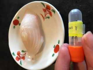
For each sample, one 1.5 ml screw-cap microcentrifuge tube was labeled with the appropriate ID code on the top and on the side of the tubes

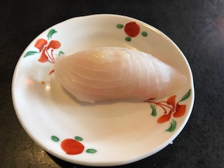
A paper plate was then divided into four sections and labeled according to the sample number. Using a scalpel and forceps, approximately 0.005g of tissue was cut from each sample on the paper plate in the appropriate quadrant. Since four different specimens were used, the scalpel and forceps with cleaned with ethanol and a Kim wipe between each fish type.

100 µl of Extraction Solution (ES) was added to each sample tube using a p200 µl micropipette with an unfiltered tip. Then, 25 µl of Tissue Preparation Solution (TPS) was added to each tube via a p200 micropipette. Using forceps, each tissue sample was added to its corresponding microcentrifuge tube.

A clean non-filtered pipette tip was used to gently mash the tissue; a clean tip was used for each tube.

The samples were left to incubate at room temperature for 10 minutes. Some tubes were left longer to incubate at room temperature as other tubes were being mashed; incubation did not start until all tubes were mashed. They were then moved to the heat block, where they were incubated at 95°C for 3 minutes.

Once the 3 minutes elapsed, the samples were removed from the heat block. Then, 100 µl of Neutralizing Solution (NS) was added to each tube. The samples were then vigorously mixed using a vortex for approximately 8 seconds per sample. Finally, the samples were placed on ice.

The next part of the lab entailed performing PCR to amplify CO1 from the fish DNA.

First, four microcentrifuge tubes were collected and each tube was labeled “1:10” along with its corresponding ID code (i.e. the first microcentrifuge tube was labeled 1:10 mh01, etc.) on the top and on the side of the tube.

In order to amplify our gene of interest, the genomic DNA (gDNA that was extracted above) was diluted using a 10x dilution. This was done to neutralize the concentration of DNA because too much DNA could prevent the PCR reaction from being performed successfully. 18 µl of purified, sterile water was added to each of the four microcentrifuge tubes just labeled. Then, 2 µl of gDNA was added to each tube. Each tube was “flicked” to ensure the solution was properly mixed.

Next, a master mix was created that included all the reagents required for a PCR reaction. Making a master mix would minimize the likelihood of errors associated with pipetting small volumes.

One master mix was made per table. Thus, for our table, the volumes of reagents listed in the master mix recipe were multiplied by 20. The reagents and volumes used to make the recipe were: 128 µl of purified water,;200 µl REDExtract – N- Amp PCR rx mix; 16 µl Forward Primer;16 µl Reverse Primer.

Then, 4 PCR tubes were labeled on the top and sides with the appropriate ID code for each sample. To each tube, 18 µl of the master mix was added. Then, 2 µl of the 1:10 dilution of gDNA was added to each tube. A sterile pipette tip was used for each sample. A negative control PCR tube was also established that consisted of 18 µl of the master mix. The purpose of this tube was to detect any amplification of gDNA that may have contaminated the master mix.

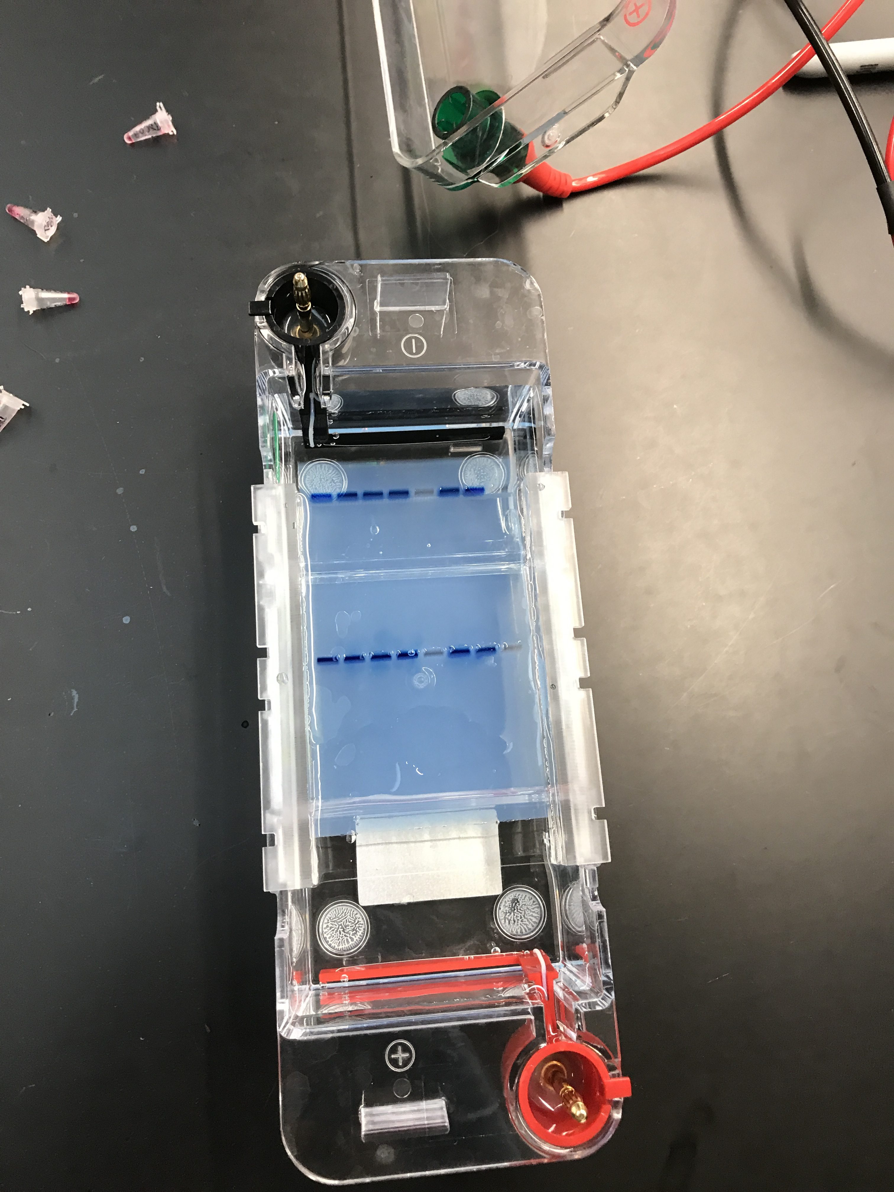
All PCR tubes (including negative control) were put in the thermocycler to allow the PCR reaction to occur. After the cycling was complete, the tubes were placed in the freezer.

A possible source of error in the experiment lied in utilizing the pipettes properly. That is, inaccurate measurements of liquids were taken, potentially affecting the volumes of reagents needed for the PCR reaction to be performed successfully.

Are sushi consumers being served the fish they ordered?

This lab investigates whether the labeling of fish in sushi on the menu is accurate or if consumers are being deceived.  Surprisingly, this has become a concern in the food scene, as some sushi restaurants are substituting expensive varieties of fish with subordinate options.

The findings presented in this lab were based on four different fish samples collected from local San Francisco sushi restaurant, New Nagano Sushi (3727 Geary Blvd. San Francisco, CA 94118).

The different types of fish samples that were collected are photographed and listed below:

Sample #1: Albacore (white tuna)

Sample #2: Hamachi (yellowtail)

Sample #3: Tai (red snapper)

Sample #4: Saba (Japanese mackerel)

Approximately 20 minutes after the fish samples were collected, they were placed in the freezer, where they were kept for 42 hours.

For our first field trip, we drove about one hour south of San Francisco along the California Coast to San Mateo County. Our first stop was Pescadero State Beach in Pescadero, CA, followed by Cowell Ranch Beach in Half Moon Bay, CA. For this field trip, we scavenged for and collected leaflets from the lupine plant that produces yellow flowers. Like other flowering plant varieties, climate and location of the plant are factors that contribute to flower color; flower color of lupines varies from yellow to violet to red and magenta.   Other important characteristics of the lupine plant include its short, bush-like stature, palm-like leaflets, and its reddish-brown stem that is most often concealed under the green foliage.

In the state, the plants are distributed along the California coast, extending from Southern California to Northern California (however, their presence is not limited to California).

As mentioned above, we first visited Pescadero State Beach in Pescadero, CA.

After a short hike along the beach, the yellow lupine plant was found along the Pescadero Marsh, just east of the State Beach.

The picture below depicts the color distinction between the lupine plant leaflets and the neighboring plant in the bottom left corner. It is clear that the leaflets of the lupine are a darker green and the plant appears to be just one shade of green, in contrast to its neighbor, which appears to have yellow and light green pigments. 

Another characteristic of the plant is the base of the flower extends just above the surface of the bush. This enables easier identification of the plant among other green plants.

We were also able to locate the lupine plant at Cowell Ranch Beach in Half Moon Bay, CA.

At this stop of our field trip, we encountered the plant at a closer proximity to the ocean than the previous site.

Below, we can clearly see the palm-like structure of the lupine plant, in which the leaflets are held together at the center and appear to bend outward.

Interestingly, the green leaflets of the Pescadero plant appeared to be slightly brighter than the leaflets of the Cowell Ranch Beach plant. A possible explanation for this observation is the latter plant was found closer to the coast, thus temperature might have influenced the plant’s development.

Conclusively, this trip stressed the importance of looking for a particular plant, given a set of features to look for that make the lupine plant distinct from other plants. Having these guidelines minimized the difficulty to locate the plant among a landscape of other plants.

Welcome to my lab notebook!

Here you find my lab entries for Molecular Ecology.