This lab is a continuation of Lab 02 and uses samples from that entry.

Materials:

• PCR tubes
• Pipette tips
• Distilled water
• Sap 10x
• SAP
• Exo
• Loading dye
• Ice
• Parafilm
• Gel electrophoresis equipment

Methods:

Part I – Gel Electrophoresis

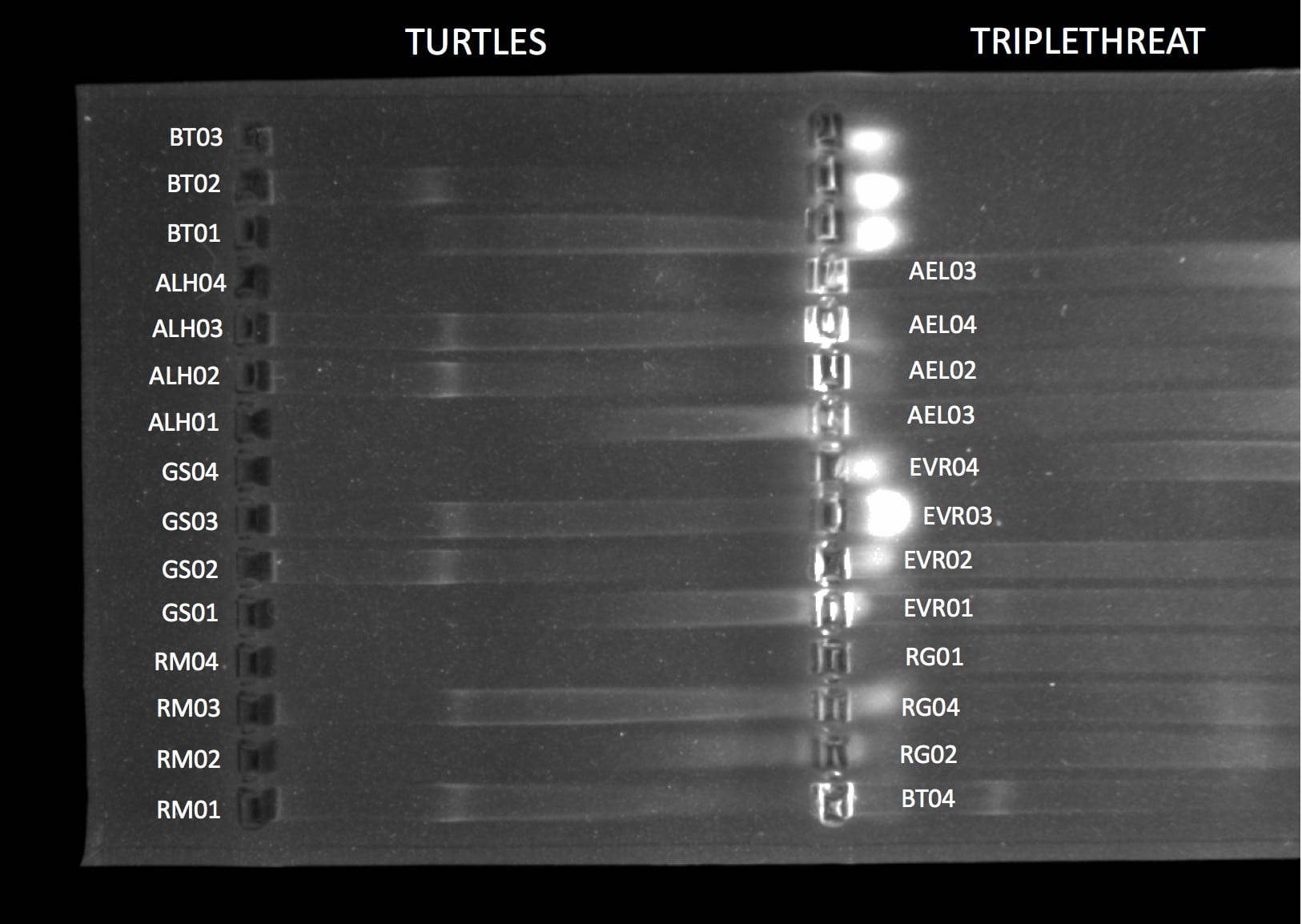
PCR tubes containing the samples labelled with EVR01, EVR02, EVR03, and EVR04 were thawed. 16 loading dye dots of about 1 uL were pipetted onto a sheet of parafilm. 3 uL of each sample was placed into its own dot. All dots were loaded into the gel alongside others’ samples as shown in Table 1. The gel was run at 130 volts for 30 minutes, which can be seen in Figure 1.

Part II – PCR Cleanup

The number of PCR cleanups that would need to be done for the products in Table 1 was calculated. Reagents were placed on ice. 7.5 uL of EVR01, EVR02, EVR03, and EVR04 were pipetted into their own 0.2 uL PCR tubes which were labeled with their respective codes. The ExoSap master mix was made using the numbers calculated in Table 2.  12.5 uL of the ExoSap mix was added to each PCR product tube. The tubes were placed into a thermocycler and the EXOSAP program was started which ran for about 45 minutes. The PCR tubes were placed into a labeled tube rack and placed in the freezer.

Table 1

Gel Electrophoresis            Template:  Genomic DNA          PCR product

Lane # (L -> R)	Sample ID #
TOP
1	Negative control
2	RG01
3	RG02
4	RG04
5	EVR01
6	EVR02
7	EVR03
8	EVR04
9	AEL01
10	AEL02
11	AEL03
12	AEL04
13
14
15	Ladder

 

Table 2

Recipe to clean-up one PCR reaction of 7.5 uL

Master Mix:                                   Rxn: 1                 Rxns: 13

H₂O                                              10.59 uL             137.67 (138)

10x buffer (Sap 10x)                     1.25 uL               16.25 (16.3)

SAP                                               0.44 uL               5.72 (5.7)

Exo                                                0.22 uL               2.86 (2.9)

Master Mix Total                          12.5 uL               162.5

PCR Product:

PCR                                                  7.5 ul

Total Cleaned-up Volume        20.0 uL

Figure 1

This class and lab period (12:45 to 17:00) was used as a time for the class to go on a field trip to Mt. Tamalpais and observe the species Mimulus guttatus and its different forms it takes. M. guttatus, also known as the monkey flower, is a plant with a wide distribution range in the United States which has various forms adapted to different areas. This particular species has yellow flowers, which implies that its pollination syndrome is by bees.

Three areas were visited to observe M. guttatus forms. The first was Cataract Bridge, a shaded trail with a small creek running through it. Alex, one of Professor Paul’s graduate students, enlisted the class’s help to collect samples from this area, which were dried in a silica gel in order to preserve them better for processing. M. guttatus “likes to keep its feet wet” which means they’re generally found in areas with moisture, where they then put down runners. When sampling, young leaves were taken from plants that were at least a meter apart to ensure they weren’t the same plant. Brief discussion of how M. guttatus seeds were spread occurred–one way was likely through water flow. This is one of the methods Alex is using in his research: how molecular ecology can be used to analyze gene flow.

Slightly up from Cataract Bridge is a field that, in the heat, was largely dried up. Despite this, we observed an M. guttatus with its seed pods. Their seeds are quite small, but M. guttatus was able to survive with very limited water in this area.

Next, we observed M. guttatus in a serpentinite patch. Serpentinite occurs in areas where two plates meet (and it’s the state rock of California!) It occasionally allows water to seep up through when it is cracked, which is where some M. gutattus patches survived.

Lastly, we walked a path to find M. guttatus in a valley. Water flows down through the valley and enables green patches to crop up–we found M. guttatus among a patch of rushes and sedges which was surprisingly muddy despite the dry grasses and buckwheat surrounding it.

Samples were obtained Monday, August 26^th, 2019 19:39 at Sakana Bune (5701 Geary Blvd, San Francisco, CA 94121) by ordering food and collecting samples in microcentrifuge tubes. Samples were stored in a freezer and thawed on September 3rd, 2019 for experimentation.

Materials

• p200 microcentrifuge
• 5 ml microcentrifuge tubes
• Razor blades/scissors/scalpels
• Heat block
• Vortex
• Ice
• Sharpie
• Gloves

Procedure

Information about the samples was recorded in a table. Each sample was given a unique code (EVR01 – EVR04) and the species name it was listed as in Sakana Bune was recorded. (See Table 1) Gloves were obtained and put on. Labelled one 1.5 ml locking lid microcentrifuge tube for each of your samples with the unique ID code with Sharpie on the side and top of the tube. A paper plate was obtained to cut samples on. Samples were cut using a scalpel in order to cut away portions in contact with other ingredients. The scalpel was cleaned between cutting each sample. Samples were cut to a size of approximately 2 mg each and added to microcentrifuge tubes with their respective labels. 100 ml of Extraction Solution was added to each tube using a p200 µl micropipette with filtered tips. 25 ml of Tissue Preparation Solution was added to the microcentrifuge tubes with the 100 ml of Extraction Solution and was mixed through gentle micropipetting with a p200 µl micropipette and unfiltered tips. Disposable micropipette tips were used by hand to mash the samples in their respective tubes. Samples were incubated at room temperature for 10 minutes and 32 seconds. Samples were incubated on a heat block at 95^o C for 3 minutes. Samples were removed from heat block and 100 ml of Neutralizing Solution was added to the samples using a p200 pipette and filtered tips and mixed by vortexing for 5 seconds each. Samples were then placed on ice.

The genomic DNA (gDNA) obtained through the above process was diluted. Labelled four microcentrifuge tubes with “1:10” and codes from Table 1 on the top and side of tubes. 18 ml of purified water was added to the tubes. Added 2 ml of gDNA to their respective tubes. Each tube was gently flicked to mix the solution.

A master mix was made to perform a PCR reaction (see Table 2). PCR tubes were labeled with the codes from Table 1 on the top and sides. 2 ml of the 1:10 dilutions of gDNA was added to each respective PCR tube, except for the negative control tube. 18 ml of the master mix was pipetted into each PCR tube and the negative control. Samples were put in the thermocycler and placed in the freezer when the cycling was complete. Settings for the thermocycler were as follows:

94^o C – 4 min (initial denaturation)

30 cycles of:

94^o C for 30 sec (denaturing)

52^o C for 40 sec (annealing)

72^o C for 1 min (extension)

72^o C for 10 min (final extension)

10^o C hold

The results of this lab can be found in Figure 1 under the heading “Triple Threat”.

Table 1

Listed Species	Code
Yellowtail tuna	EVR01
Salmon	EVR02
Mackerel	EVR03
Bluefin tuna	EVR04

 

Table 2

Reagent                                                  Volume (1x)       Master (volume x 13)

Water (PCR Quality)                              6.4 ml                  83.2 ml

REDExtract-N-Amp PCR rx mix           10 ml                   130 ml

Forward Primer                                       0.8 ml                  10.4 ml

Reverse Primer                                        0.8 ml                  10.4 ml

Tissue Extract (gDNA- 1:10 dilution)    2 ml                     ———

Total Volume                                         20 ml                   234 ml

 

Figure 1