October 8, 2019
In Lab Portion:
To prepare for this lab, we were assigned the task of assembling an alignment of COI sequences that includes our fish DNA barcode sequences and sequences downloaded from NCBI through Geneious. Once we had this alignment, we were told to use the ‘allow editing’ tool to ‘clean-up’ our alignment so that all the sequences begin and end at the same point. When I looked through the first 20 columns of my alignment, I found only one column that showed a polymorphism.
Choosing the best model of molecular evolution
Next, we used a program called jmodelTest2 to establish the best model of molecular evolution for my sequences. Within the folder called “jmodeltest-2.1.10.tar.gz” there was a file named ‘jModelTest.jar’ that opened a window. Before using the jmodelTest2, we had to return back to the Geneious program and export the alignment in Phylip format (relaxed). Once that was completed, I could go back to the jModelTest2 and open the exported alignment. We then were able to compute the likelihood scores’ of each model of molecular evolution as the program goes through a set of hierarchal set of 88 models based on an initial tree that it uses for all tests.
Once the likelihood calculations were completed, we used two methods to choose the best model based on some optimality criterion. The two methods were the Akaike Information Criterion (AIC) and the Bayesian Information Criterion (BIC). The best model based on AIC was model 79. Similarly, the best model based on BIC was model 79.
Bayesian Inference
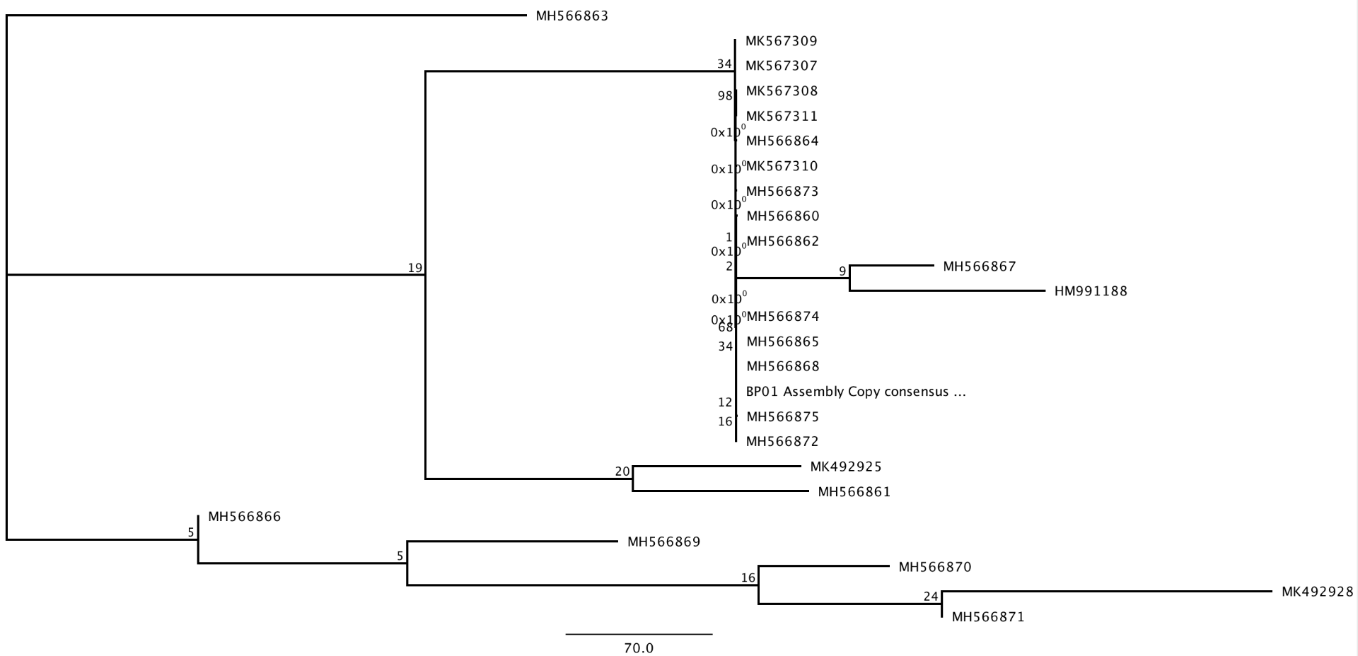
Back in Geneious, we were able to install the ‘Mr.Bayes’ tab by using ‘Tools’ > ‘plugins’ in the menu bar. We selected our alignment and chose Mr.Bayes as our ‘tree’ of choice. In the settings, I chose to use the GTR (complicated) substitution model as my model of molecular evolution that was closest to my jModelTest complexity. Next, I chose to set my ‘rate variation’ to ‘gamma’ because my jModelTest best model contained a ‘+G’ in it. The outgroup that I chose for this alignment was a shark species under the consensus identity #HM991188. Under the MCMC settings, I chose a ‘chain length’ of 10,100, a ‘subsample frequency’ of 200, and a ‘burn-in length’ of 100,000. Under the ‘Priors’ settings, we used ‘Unconstrained Branch Length: Exponential (10)’ and ‘Shape Parameter (10)’ which affects the shape of the prior statistical distribution. The Posterior distribution showed that this analysis was not run for long enough. The Trace figures showed an upward sloping line that is representative of an increase in the posterior probability and is part of what you want to remove with the burn-in length. We ran our analysis one more time but used a ‘chain length’ of 110,000 and 10,000 for the ‘burn-in length’ this time. With this second run, we found that the Posterior distribution was normal and the Trace figures looked like the ‘fuzzy caterpillar’. I recovered the same clades in my tree and they both had similar support values.
Maximum Likelihood
In this last section, I used maximum likelihood to infer a phylogenetic tree of my aligned data set. First, I went the menu bar and through ‘Tools’>’Plugin’, I was able to install RAxML which does a very fast maximum likelihood inference. For the evolutionary model, I chose ‘Rapid bootstrapping’ and run the it. Once the process was finished, I built a consensus tree by selecting the ‘RAxML bootstrapping trees.’ I found that the clades with high support do not match those from your bayesian analysis.
Next, we used a different program that uses maximum likelihood called ‘PHYML.’ We ran this analysis with bootstrapping and we used the HKY85 model of molecular evolution for this and our final Bayesian Tree.
Results from our ‘In Lab’ portion:
At Home portion:
Our Assignment for the second portion of this lab was to use the same alignment and the HKY85 model of molecular evolution to infer my best tree using Mr.Bayes. For this run the only modified setting were the ‘chain-length’ was set to 3,000,000, the ‘burn-in length’ at 300,000, the ‘subsample frequency’ at 500. This run lasted for about 5 hours long!
Result from our ‘At Home’ portion:

