11/14/18 Wednesday ISSR Analysis and Geneious.

I added loading dye into my PCR tubes, which were used from last lab. I added about 1 micro liters to each tubes (15 total).

Then including the solution inside the PCR tube, total of 5 micro liters, I added into the agarose gel that was given by the professor. The first and last wells were saved for ladder. I added 15 of Carter’s samples first and added my samples second. Kayla added her samples and added 3 of Peter’s samples. Last of Peter’s samples (12 samples) were loaded on the lowest line of 50 wells.

After every table loaded their samples onto the wells, professor Paul ran these gels at a low voltage (20 volts) for a long time ans see how things turn out. We didn’t get to see what happened.

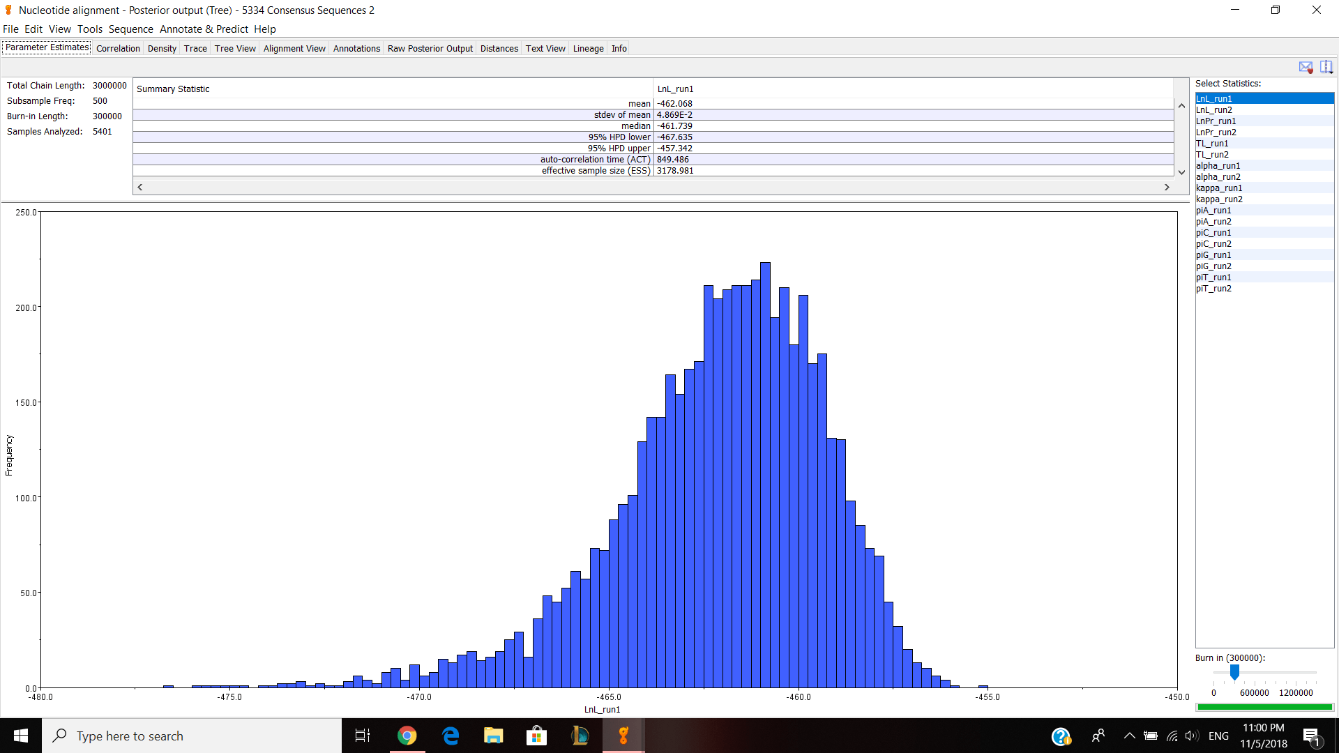
Next, we moved on to Geneious. Our table had to do some work with JP5551 because our previous JP5334 was not very good. I did the same thing with JP5551 from the last lab and sent it to professor Paul so that every can download my nucleotide alignment and make concatenated alignment. I made a separate concatenated file and put JP 5334,5551,5525 and 5536 into the file. Then I choose all four documents and choose tools>Concatenate Sequences or Alignments and clicked ok. It created a concatenated alignments and I opened up to see if it looks correct. I have about 1500 nucleotides and I edited/cut the alignment 1029-1085 because it looked bad and thought that it can effect my phylogenetic tree. Next, I exported the file in phylip alignment type and saved it. Then I opened jmodeltest and loaded my alignment and compute likehood scores to calculate AIC and BIC. I got TPM G for both AIC and BIC so for my Bayesian analysis, I chose HKY85, gamma and TG0248. Then ran the analysis for 3,000,000 chain length, 500 subsampling frequency and 300,000 burn in length values. It took about 2 hours and 30 minutes and gave me this result.

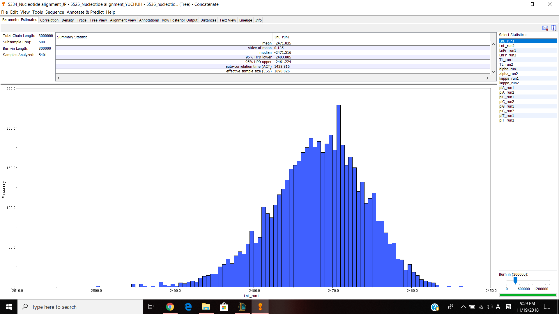
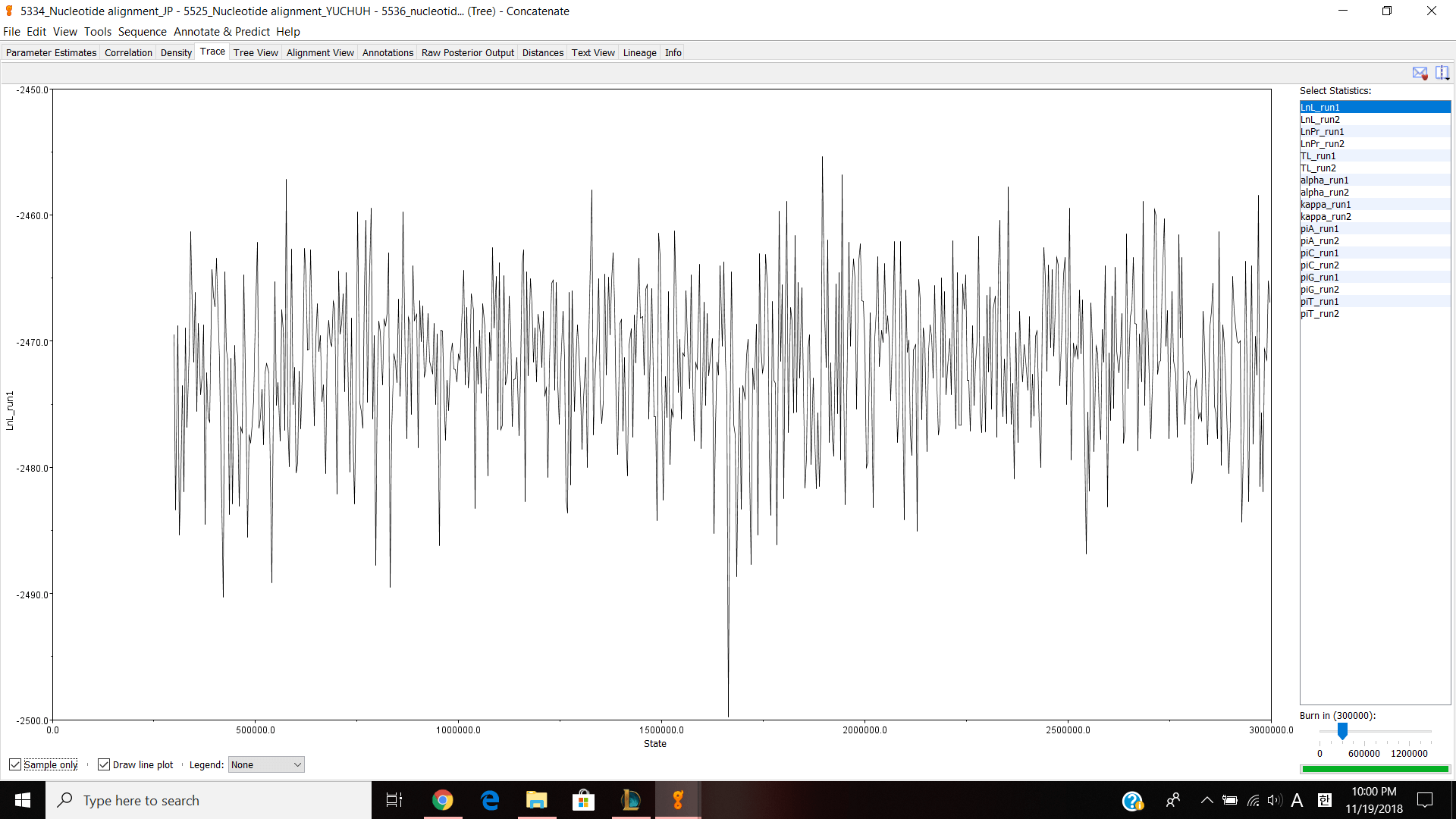
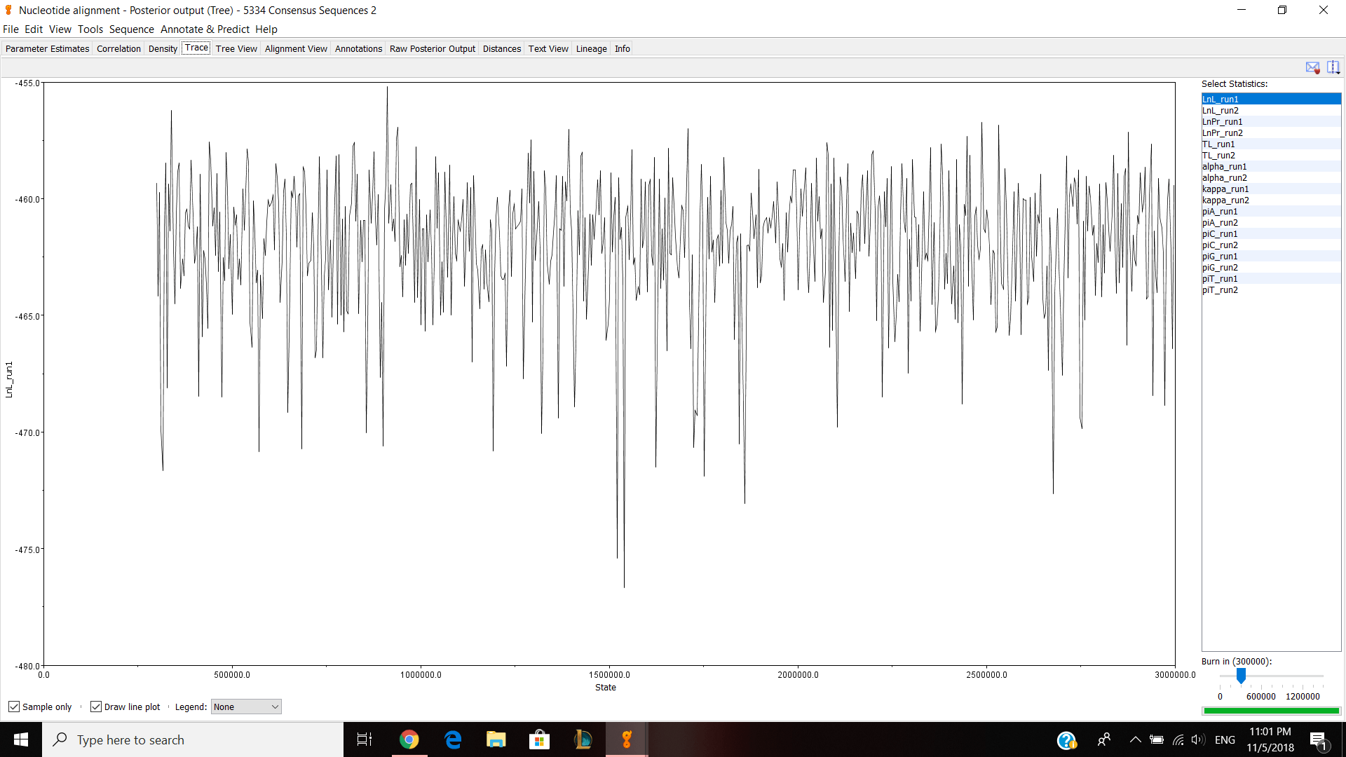
Parameter estimates look pretty good and the trace graph has that caterpillar thing shown on the graph.

This is my tree view. My tree included multiple clades with the support value that is greater than 0.85. And I think that these individuals within in each clade are found in the same population.

I think that these concatenated EPIC markers provided enough resolution to distinguish populations phylogenetically  because we, as a class, gather 4 different primers to make 4 different nucleotide alignment making it more precise and accurate than using just one primer. My analysis couple weeks ago was on JP 5334, which is the weird one, so I don’t know if it came out correctly, but it looks like I have a little more resolution than the single marker analysis on JP 5334 couple weeks ago.

11/7/18 Wednesday Plant DNA PCR-ISSRs

Professor Paul ran our Genomic DNA of the samples from last class, several samples were successful and some weren’t.

In this lab, we used two interspersed-simple-sequence-repeat (ISSR) primers in PCR reaction. We used samples of Lupinus arboreus samples from last years class. It was the same species that we saw in our field trips.

First, I made 1:10 dilutions of 5 Lupinus arboreus samples. Three 1.5 mL tubes with unique ID. I pipette 45 micro liters of water and 5 micro liters of each samples into each of the three 1.5 mL tubes. Then I put total of 15 tubes into a rack so that every table gets the diluted samples.

After everyone was done with dilution, I grabbed 15 diluted tubes: PRL 01,PRL 02, PRL 03, PRL 04, PRL 05, PRM 01, PRM 02, PRM 03, PRM 04, PRM 05, PHT 01, PHT 02, PHT 03, PHT 04, and PHT 05. I then grabbed two 0.2 ml 8-tube strips (PCR tube strips) that I will be using for the 15 reactions per marker. I wrote sample ID, primer number (17898) and my initials. I then using filter tips, I pipette 1 micro liter of my first template DNA (dilution) into the first tube of my PCR strips that I labeled. I continued this step and changed the tips everytime I changed my samples. After I was done transferring 1 micro liters each into 15 PCR strips, I put them on ice.

Kayla V. then created Master Mix for our table. Our Master Mix was based on per 80 reactions so the measurements were ddh2o=1000 micro liters, 10x buffer +mg=240 micro liters, BSA=80 micro liters, dNTPs=160 micro liters, Primer (17898)=20 micro liters, Taq=20 micro liters and my template=1 micro liter. Total of 1520 except the amount of my template DNA.

After she was done creating the Master Mix, I pipette 19 micro liters of the Master Mix and added to each of the PCR strips adding up to 20 micro liters into each PCR strips. Every time I added the Master Mix, I mixed the solution by gently pipetting up and down.  After pipetting in 19 micro liters of the Master Mix into each PCR strips (15 time), I closed the lid tightly and put them into the PCR machine.

That was the end of the lab on Wednesday.

10/31/18 Wednesday. In this lab, I used Geneious to code heterozygotes and find polymorphism in the sequences.

Our EPIC marker failed, EPIC failure haha. So we used last year’s data, which were 5334 forward and reverse reads (25 reads of Mimulus cardinalis and outgroup of Mimulus lewisii).

First, I created forward and reverse sequences folder and dropped the reads into the file. I downloaded the reads from Canvas. Next, I selected all the sequences, both forward and reverse reads, and build an alignment using Muscle (default setting). Then, I looked at my nucleotide alignment and cut the ugly reads and looked for polymorphism and heterozygotes. I found many polymorphism and misreads, but about 10 true heterozygotes. Only 4-5 were true heterozygotes and polymorphic. I recoded the true heterozygotes with the appropriate ambiguity code from the IUPAC Ambiguity Code list I have been given in the beginning of the class. After I was done editing, I saved and applied the changes. Next, for each Forward and Reverse pair, I De Novo Assembly them and edited the assembly document so that it has good reads and correct Ambiguity Code. I repeated the same step from another pairs except the outgroup (TG0248) and forward read that did not have a pair (JP 1132). Then, I selected all the Assembly files and generate consensus sequence, and create sequence list. I then extract sequences from list and created a subfolder named 5334 Consensus Sequences. This will move all my Assembly documents into this subfolder. I then manually moved my outgroup reads and JP 1132 reads. Next, I selected them all and choose Edit, Batch Rename and click Remove button and put 33 to remove all the characters except the sequence name for the selected documents. However, I had to edit the name of the outgroup and JP 1132 by hand. After that, I selected all and created alignment using Muscle. I opened the alignment and did some trimming.

AT HOME – INFER A BAYESIAN TREE OF THIS SINGLE LOCUS ALIGNMENT:

I inferred a Bayesian phylogenetic tree using  5334 nucleotide alignment and used the outgroup TG0248 and ran it for about 1hour and 30minutes. This is what I got after the run:

Left is the parameter estimates and right is the trace (good fuzzy caterpillar).

Tree 5334 consensus sequence-2krc97c

If screenshot the screen and paste it here, it came out blurry, so I just created a link to the Bayesian phylogenetic tree of 5334 consensus sequence.

10/24/18 Wednesday, we continued our DNA extraction (plant) by running the genomic DNA gel. Just like with the fish genomic DNA gel, Kayla dropped total of 12 loading dye drops about 1 micro liters and on top of that dropped 12 3 micro liters of our genomic DNA. And then dropped total of 4 micro liters of the mixture into the well. First three was Kayla’s, Second three was Carter’s, Third three was Peter’s and Fourth three was mine. Gel was ran for about 20 minutes at 140 voltage. After 20 minutes, I took out the gel and put it into the machine to see our DNA on the gel. My JP 1303 failed and Kayla’s JP 1317 failed. So Professor dropped 4 total samples which were JP 1317, 1303, 1290, 1300. Here are the pictures of our genomic DNA gel run result.

Total of 32 tubes were given on each table and all tubes were the same. I took 8 tubes, which are JP 1292, 1295, 1299, 1302, 1304, 1308, 1314, and 1316. Next I labeled 0.2 ml 8-tube strips (PCR tube strips) that I will be using for the reactions (labeled sample ID, date, and the primer number). And using filter tips I pipette 1 micro liter of my template DNA into the tubes (total of 8). I changed tips every time I used one to avoid contamination. After eight 1 micro liter of my sample genomic DNAs were placed into the right eight tubes, I placed it on ice. While my samples were on ice, I had to make enough Master Mix for my table.

To make Master Mix, I added 600 micro liters of ddH2O, 80 micro liters of 10x buffer +Mg, 40 micro liters of BSA, 8 micro liters of dNTPs, 8 micro liters of both F-primer 5334 and R-primer 5334, and 1.6 micro liters of Taq. So total of 745.6 micro liters. To mix it well, I spun down the tube briefly.

Once the Master Mix was made, I took out my 8 PCR tube strips from the ice and added 19 micro liters of Master Mix into each of my samples (total of 20 micro liters inside each PCR tube strips). After all my classmates were done with this step, Professor Paul placed our PCR tubes in the PCR machine and closed the lid.

10/17/18 Wednesday. Wet lab: population Genetics project- DNA extraction (plant) and Gel Electrophoresis 1

In the beginning of the lab, I received a sheet of paper with the title Plant Tissue DNA Extraction and table consisted with Sample ID, Location and Species. Then I received three samples from Prof. Paul and those were JP 1319 mill creek mono north M.guttatus JP 1303 and JP 1296.

Modified Alexander et al. tube protocol for DNA extraction

Note: Always use filtered tips for all steps in this protocol.

First, I labeled my given 3 2.0mL tubes with my sample ID (JP 1319, JP 1303 and JP 1296). Then I added three sterile 3.2mm stainless steel beads to each tube. Next, I took my tweezers and took out my sample leaf tissue, the size of my thumb nail, and put it into the given tubes with the label. I cleaned my tweezers with ethanol every time I took out different sample leaf tissue. As a group, Peter loaded the tubes within a tube rack into the modified reciprocating saw rack and mount the rack into the saw. He pulled the trigger and let the machine shake for 40 seconds. This process is to mush the leaf tissue and make it like a powder like. After 40 seconds, as a group again, we put each of our samples and briefly spin down the tubes in the centrifuge for about 30 seconds at the maximum speed to pull plant dust down from the lids. I then took out my sample tubes and added 434 micro liters of preheated grind buffer to each tube. After that, I incubated buffered grindate at 65 degrees Celsius for 10 minutes in water bath, mixing the tubes by inversion every 3 minutes. After 10 minutes, I took out my sample and added 130 micro liters 3M pH 4.7 potassium acetate, invert tubes several times and incubate on ice for 5 minutes. I waited for the entire class to start centrifuging at the same times. After everyone was done, as a group, we put our samples in the centrifuge and spun it at maximum force for 20 minutes. While it was getting centrifuged, I labeled new 1.5mL tubes with the sample ID (top and side). I also labeled Epochspin column tubes (blue on the bottom, white with filter on the top). I will be adding supernatant and it will capture DNA and filter out the waste. After it was centrifuged, I transferred my supernatant (on the top) to these sterile 1.mL microcentrifuge tubes. After transferring my supernatant, I added 450 micro liters of binding buffer into JP 1319 and JP 1303 and added 600 micro liters of binding buffer into JP 1296. I then added 650 micro liters of each mixtures to each of Epoch spin column tubes (correctly labeled ones) and centrifuged it for 10 minutes. After it was done, I dispose the buffer (in the blue tube) into the hazardous waste bottle and repeated the same thing again. After centrifuging all my mixtures, I added 500 micro liters of 70% EtOH to the column and centrifuged for 8 minutes and discarded the flow-through. EtOH is to wash the DNA bound to the silica membrane. I repeated the same thing again and at the third time I centrifuged for 5 minutes without adding anything in the column to dry out any residual ethanol. I labeled another 1.5 mL tubes with sample ID and date, which will hold my final extracted DNA. After ethanol was all dried up, I threw out the blue bottom and switched with 1.5 mL tubes. I then added 100 micro liters of preheated (65 Celsius) pure sterile H20 to each tube, let it stand for 5 minutes and centrifuged for 2 minutes to elute the DNA. After it was centrifuged, I threw away the column (top), capped the bottom and put it into the ice box.

10 October 2018, Wednesday. For last week’s lab HW, I had to make a folder with three of my samples (CO-01,02 and 03), 25 sequences of the COI gene for Actinopterygii and at least one COI gene for Chondrichthyes (outgroup). To find those sequences, I had to log into Geneious and click NCBI nucleotide section and then type in COI Actinopterygii or Chondrichtyes on the search bar. I put all 29 samples into one folder and made an nucleotide alignment sequence.

Phylogenetic Inference

First thing that I did was to clean up my alignment to begin and end at the same point. I just clicked ‘Allow editing’ and select the bases and deleted them. Looking at the first 20 columns of my alignment, I found 12 polymorphic nucleotides. Next I downloaded JModelTest2 from Canvas. I had to download Java to open up the file jmodeltest2 because my computer was not able to open up the file. After that, I went back to Geneious and export my edited alignment in Phylip format (relaxed) by choosing Export, selected documents’, ‘Phylip’ file type and relaxed Phylip file at the end. And using JModelTest 2, I opened up the exported alignment. Next I chose ‘Analysis > Compute likelihood scores’ from the menu. My alignment took about 5 minutes for the program to look for the likelihood for each of the models to be the best fit. After the calculations were done, I looked up AIC and BIC values (red, top scoring model) and found out that the values were the same with HKY +G.

Bayesian Inference

Back in Geneious, I clicked Tools, Plugins and install the Bayes plugin. Then selected my alignment, right click and chose Tree then MrBayes. Changed the substitution Model to HKY, Rate Variation to Gamma, Outgroup to shark, Chain length to 10,100, Subsample frequency to 99, Burn-in Length to 100 and left the heated chains at 4. I then run the analysis and didn’t took that long. Double-click on new ‘Posterior output’ to open up the result and click on the ‘parameter estimates tab’. I got really bad graph as expected and also got bad Trace as expected because the run time was very fast. This time I changed chain length to 100,000 and bur- in length to 10000. It took about 10 minutes and I got a pretty good graph.

Maximum Likelihood

This time, I went to Tools, Plugins and installed RAxML. This time, instead of choosing Bayesian, I chose ‘Rapid bootstrap with rapid hill climbing’. Once RAxML was done, I clicked ‘RAxML bootstrapping trees and right clicked to choose Tree and consensus tree builder. After that I chose ‘Create consensus tree’ and ‘Support threshold’ of 50%, and then ‘ok’. I had a decent tree and for my report I had to take two sequences out because the branch was too long. The other steps didn’t work so i had to stop at PHYML part.

10/3/18 Wednesday. Today, I used Geneious to look at my forward and reverse reads, however my reads weren’t successful so I had to used the given three forward and reverse reads which are CO-01-Albacore, CO-02-Big eye tuna and CO-03-Yellowtail.

I received “An Introduction to Geneious” handout with instructions on how to use Geneious and do the exercises. I first downloaded all the forward and reverse reads and drop the file into the folder that I named “Jinwoo Kim DNA barcoding for Molecular Ecology”. Next, I looked both forward and reverse reads to see how good they were and the HQ% was around 90s so they were very clean. Using CO-01, I tried looking at the sequence by clicking sequence view and also tried editing the nucleotide bases and etc… but never saved it. After that I copied the reverse sequences CO-01 into the forward reads folder. I then selected both of them and right clicked to choose ‘De novo assembly’ to assemble the two reads. Next, I clicked the created file named ‘assembly’ and zoom in to see the overlap of reverse and forward reads. Mine had high HQ% values so I was able to cut the ends of both sequences and was good to go. After the trimming the mess, I saved the file and choose ‘Generate consensus sequence’ and clicked ok. I BLAST the assembly ‘consensus sequence’ and resulted to have scientific name of the organism that has the highest matching sequence to mine. I searched up the scientific name to see if its the correct fish. At last, I copy and paste 5-7 alignment to my created folder named “Fish barcode test alignment’ and selected them all to click ‘Multiple align’ and get a new ‘nucleotide alignment file’. I followed this steps for CO-02 and 03.

Exercises:

1. CO-01—– Matched, Albacore=T.alalunga,  CO-02—–Matched, Big eye tuna=Thunnus albacores, CO-03—–Matched, Yellowtail=Seriola quin queradiata.
2. CTTTTCTGATG (first 10) and total of 18.

26 Sept. 2018 Wednesday

Our last field trip was to Mt. Tamalpais and the weather was hot and cold in between each stops. We first stopped at where I believe it was Alpine Dam and we walked down the trail and stopped at one point where there was little river and had to go through little adventure (and I got hurt little bit). Few of us went down to the river and saw some plants between rocks and also saw bunch of ladybugs having a party inside a bush. Here are some pictures.

After some adventure, we drove across the bridge and went up the mountain and stopped at a place where plants were growing on wet grounds. Here are some pictures:

Professor has told us that this kind of plants need to be on wet ground all the time.

Next we drove down to the coast to see the purple-flowered lupine that was the same but different color from last field trip to Pescadaro state beach. As we drove to the coast, the view was so good that I had to take a picture of it.

Anyways, we dropped at one point where we observed purple-flowered lupine and it was in similar environment as the yellow colored lupine. There weren’t a lot of them, but we were able to find pea-shaped flowers, immature fruit and old fruit. We even found one on the cliff that was growing on top of the rock. It was windy and cold and there were lot of birds creating white rock. I was thinking that these species might have been spread out due to the wind and maybe the birds. Here are some pictures of the flower:

From this field trip, I was more amazed by the nature than the field trip from last week. It was amazing how we were able to find the same species but different color that is 2 hours apart from each other.

p.s Sad that this was our last field trip as a class 🙁

9/19/18 on Wednesday it was a windy and sunny day at the pescadero state beach.

It was about an hour drive to the beach and after we stopped at the pesacadero state beach, we saw old fruit of Lupinus arboreus along the sea side. Here is the picture of it.

Then we walked down the bridge and found more Lupinus arboreus. We observed immature fruit and pea-shaped flower of Lupinus arboreus.

left is the immature fruit of Lupinus arboreus and right is the pea-shaped flower of Lupinus arboreus.

We weren’t able to look around more because the drive was too long.

Hope, our next field trip go well and observe more of these living things out there.

-Jinwoo Kim

9/12/18

Continuing on with our experiment, I started with running the PCR products on gels. It was the same procedure as from the last week’s lab. I made array of 2µl dots of loading dye onto the Parafilm and made total of 12 dots for my lab group. And on top of the loading dye, I added 3µl of PCR product from the top to bottom: Kayla, Carter, Peter, and Jinwoo. After that I loaded the gel along with the latter and recorded the location of my PCR product.

After Gel electrophoresis was finished, we checked our genomic DNA and unfortunately, I couldn’t see my DNA on the gel. So… I made another master mix and using my gDNA, I created another PCR product so that Professor Paul can get my genomic DNA for DNA barcoding.

If my genomic DNA were to be shown on the gel, I would have done ExoSap PCR clean up.

Materials for ExoSap PCR clean-up:

-H2O

-10x buffer (Sap 10x)

-SAP

-Exo

-Ice

-Thermocycler

Procedure:

First, I was suppose to determine the number of PCR clean-ups that I have to do and calculate the volume of Master mix needed for my PCR. Then Pipette 7.5µl of each PCR product into a clean, labeled 0.2µl PCR tube and put it into a bucket of ice while making the ExoSap master mix. After making master mix, pipette 12.5µl of master mix into each PCR product tube (3 total if you had 3 genomic DNA found). Next, I would have placed the tubes in a thermocycler and start the ExoSap program. After the program is completed (~45 minutes) place PCR tubes in a labeled tube rack and place in the freezer so that it can get sent to somewhere that can do DNA barcoding.

p.s. I don’t know if my PCR product succeeded or not.