Category: Uncategorized

We conducted a double digest restriction associated DNA (ddRAD) study on Mimulus guttatus.  The 1st step was collecting samples which was done on two field trips that can be read: https://usfblogs.usfca.edu/mkmin/wp-admin/post.php?post=23&action=edit. 

Next, we extracted DNA from the samples collected as well as samples previously collected by the graduate student, Alex: https://usfblogs.usfca.edu/mkmin/wp-admin/post.php?post=23&action=edit. 

Next, we double digested our DNA using two restriction enzymes:  https://usfblogs.usfca.edu/mkmin/wp-admin/post.php?post=23&action=edit.  These enzymes cut out the genome into many pieces. 

The unique DNA barcodes were ligated onto each of the individuals.  PCR was used to add a 2nd unique barcode and test if the library construction was successful.  Our PCR was successful, which was photographed by Professor Paul.  After the test PCR, a larger reaction was conducted  (assumed it was successful since 1st one worked).  This was the last step we were able to do as a class.

The next step would be size selection which selects DNA of specific sizes, specifically, we would target from 400-600 bp fragments to use with the Illumina technology.  Size selection can be done in 3 ways by using an automated system called Pippinprep of which we have one in the Suni Lab.   Another way is to use gel extraction (run out full product of PCR and cut out) or use magnetic beads to isolate the DNA fragments.  After size selection, we would then normalize our DNA samples which brings DNA samples to approximately the same concentration.  The number of DNA fragments will be sequenced.  Finally, the last step would be to combine the size selected and normalized PCR products into one vessel.  Then, we would run these samples on any Illumina sequencer (iSeq 1000).  Sequencing would take about 16 hours and if successful, would generate tens of millions reads of the data.  These data would be thrown into a bioinformatics pipeline.  Ultimately, we would align the sequence data with the published Mimulus guttatus genome and call SNPs.  The SNP’s would be used to infer population differentiation using a metric-like FST and access population genetic diversity, such as looking at the number of alleles, allelic diversity, etc.  Based on what I know about Mimulus guttaus, I would expect populations that are geographically divergent to also be genetically divergent.

Lab: Tuesday, 9/24/19

Location: Mt. Tamalpais

• Saw flowering population of mimulus that had really big flowers by the mountain water and stays moist throughout the summer.

 

Redwood Creek Mimuli

• Dynamic place
• Very low population density of mimulus
• Gene flow and seed flow were both primarily downstream
• Unlikely getting cues to flower with a very minimal interaction
• Conservation

DNA Extraction protocol: 

1. Labeled 3 2.0 mL with my sample codes: Tube #1 MM CATB, Tube #2 MM LOTR003, Tube #3 SCHO 003.
2. Added 3 sterile 3.2 mm stainless steel beads to each tube.
3. Added a small amount of leaf tissue to each tube – be sure to clean any tweezers or scalpels used between tubes to avoid cross-contamination.
4. Loaded the tubes within a tube rack into the modified reciprocating saw rack and mount the rack to the saw.
5. Spun down the tubes in the centrifuge (15-2o seconds at fast speed) to pull plant dust down from the lids.
6. Added 434 µL preheated grind buffer to each tube.
7. Incubated buffered grindate at 65C for 10 minutes in water bath, mixing the tubes by inversion every 3 minutes.
8. Added 130 µL 3M pH 4.7 potassium acetate, inverted tubes several times and incubated on ice for 5 mins.
9. Spun in the centrifuge at maximum force for 20 min. This will be 14,000 or 15,000 rpm for the tubes in a small microcentrifuge.  Be sure to balance the microcentrifuge.
10. Labeled new 1.5 mL tubes with the sample ID.  Transferred supernatant to these sterile 1.5 mL microcentrifuge tubes.  Avoided transfer of any precipitate.  The precipitate will be fairly obvious and looked like small green particles on the bottom of the tubes or plate wells.
11. Added 1.5 volumes binding buffer.  Typically ~400 µL is recovered from previous steps, in which case 600 µL binding buffer is added.
12. Applied 650 µL from Step 11 to Epoch spin column tubes and centrifuged for 10 minutes (until all liquid has passed through) at 15,000 rpm in a centrifuge and discarded flow-through.

• Disposed this buffer

13.  Repeated step 12 with the remaining volume from step 11.

14. Washed the DNA bound to the silica membrane by adding 500 µL of 70% EtOH to the column and centrifuge at      15,000 rpm until all liquid has passed to the collection tube (8 mins).  Discarded the flow-through.

15. Repeated step 14.

16. After discarding the flow-through from step 15, centrifuged the columns at 15,000 rpm for an additional 5 min to remove any residual ethanol.

17. Discarded the collection tubes and placed the columns in sterile 1.5 mL microcentrifuge tubes.  *Made sure these 1.5 mL tubes are labeled with Sample ID and date — hold your final extracted DNA.

18. Added 100 µL preheated (65C) pure sterile H2O to each tube.  Let stand 5 minutes and then centrifuged for 2 mins at 15,000 rpm to elute the DNA.

Tues, October 30th 2019

Gel Electrophoresis/PCR Cleanup

Gel Electrophoresis of PCR products:

1. Grabbed PCR tubes from ice and thawed
2. Dotted out 12 loading dye dots (2µL) on a sheet of parafilm
3. Pipetted 3 µL of each PCR product into its own dot
4. Loaded all the dots into the gel (7 µL each)
5. Ran the gel at 130 volt for 30 minutes

Tues, November 5th 2019

PCR Reaction 

Made up a Master Mix per table: *multiplied everything by 18

*Followed the protocol

Reagent                          Volume  (µL)

ddH2O                             240.48

10x Buffer                       36

MgCl2                              36

BSA                                  18

dNTPs                              3.6

F-primer                          3.6

R-primer                          3.6

Taq                                    0.8

Template                          n/a

Total : 20 mL per rxn

Tubes                 Specimen ID 

QS1                       MM1

QS2                      MM2

QS3                      MM3

QS4                      OY01

QS5                      OY02

QS6                      OY03

QS7                      EB

QS8                     RDRK001

QS9                     SHOR005

QS10                   KRS1

QS11                    KRS2

QS12                    KRS3

 

Tuesday, November 12th 2019

DD-RADSeq (Double-digest restriction associated DNA sequencing) 

I. Double Digest

1. Double digested 100-1000 ng of high quality genomic DNA with selected restriction enzymes.  A digestion buffer was used for both enzymes.
2. Placed 6 µL of each sample’s DNA in the PCR tube, stored on ice.

Sample #1: MONO 006 10

Sample #2: CHIM 005 5

3. Prepared Master Mix 1:

Added 3 µL of the Master Mix 1 to each sample’s DNA.   (11 rxns)

CutSmart buffer 10x     0.90 µL x 11 = 9.9 µL

EcoRI-HF enzyme        0.28 µL x 11 = 3.08 µL

MSPI enzyme                0.12 µL  x 11 = 1.32 µL

Pure water                     1.70 µL x 11 = 18.7 µL

Master Mix total: 3 µL  x 11 = 33 µL

4. Sealed the samples, vortexed, centrifuged, and incubated at 37C for 8 hours on a thermocycler with a heated lid                set to 50C.

II. Adaptor Ligation

1. Thawed the working stock EcoRI and MspI adaptors made previously.

Sample #

1 – 17: Eco-2

1- 18: Eco-2

1 – 19: Eco-3

1- 20: Eco-3

1 – 21: Eco-4

1- 22: Eco-4

1 – 23: Eco-5

1- 24: Eco-5

2. Added 1 µL of the working stock EcoRI adaptor directly to the digested DNA.

3. Prepared Master Mix 2

Added 3 µL of the Master Mix 2 to each sample’s digested DNA.   (11 rxns)

CutSmart buffer 10x     0.40 µL x 11 = 4.4 µL

ATP (10 mM)                 1.30 µL x 11 = 14.3 µL

T4 Ligase                        0.20 µL  x 11 = 2.2 µL

Pure water                     0.10 µL x 11 = 1.1 µL

Universal P2 MspI adaptor 1.00 µL x 11 = 11 µL

Master Mix total: 3 µL  x 11 = 33 µL

4. Sealed the samples, vortexed, centrifuged, and incubated at 16C for 6 hours on a thermocycler with a heated lid                set to 50C.

 

Tuesday, November 18th 2019

DD-RadSeq (PCR Test of Successful Library Construction) 

I. Test PCR

Tested for successful library construction of Mimulus gutattus samples (restriction digest and barcode ligation) using a test PCR.

Steps

PCR I will test for the success of library construction and can be performed with inexpensive non-high-fidelity Taq.

1. Prepared a Master Mix for one PCR reaction of 16.0 µL

Master Mix:                                   Rxn: 1                            Rxns: 11

NEB One-Taq 2x Master Mix     8.0 µL                           88 µL

Forward Primer (10 mM)           0.40 µL                         4.4 µL

Reverse Primer (1o mM)            0.40 µL                         4.4 µL

Pure H20                                       6.2 µL                            68.2 µL

Master Mix Total                         15.0 µL                           165 µL

Library DNA Template              1.00 µL

Total rxn volume                         16.0 µL

Test Samples: 17, 18, 19, 20, 21, 22, 23, 24

2. Ran the PCR using “PCR1” on BIORAD #1/2 (BIORAD #1/2 → DDRAD → 2_PCR1; the       folowing conditions on a thermocycle with a heated lid: 94C for 30 sec, 60C for 30 sec, 68C for 45 sec).  4-10C infite hold.  

3. Ran the products of PCR I for each sample on a 1.5% agarose gel (0.75 g agarose in 50 mL 1x TAE) with a 100 bp ladder at 130V for 40 minutes.

 

II. Final PCR (PCR 2)

This PCR run added the special ‘second barcode’ sequences and Illumina primer to Mimulus gutattus, allowing to identify which specific individuals in a given sequence comes from (Ligation barcode + PCR2 barcode).  Each table used a different PCR2 primer.  Our was PCR2_1.  A PCR amplification was done with a Phusion Polymerase kit and added Illumina flowcell annealing sequences, multiplexing indices, and sequencing primer annealing regions to all fragments and to increase concentrations of sequencing libraries.

1. For each library, 4-8 PCR reactions were set up in 50 µL total volume and prepared a Master Mix for one PCR reaction of 25.0 µL

Master Mix:                                   Rxn: 1                            Rxns: 11

Phusion DNA Polymerase          0.31 µL                           3.41 µL

5X Phusion HF buffer                 6.25 µL                         69 µL

Forward Primer (1o mM)          1.56 µL                           17.16 µL *PCR1_X)

Reverse Primer (10 mM)           1.56 µL                           17.16 µL *PCR2_1

DNTPs (10 mM)                          0.63 µL                          6.93 µL

DMSO                                            0.94 µL                          10.3 µL

Pure H2O                                      10.75 µL                         118 µL

Master Mix Total                         22.0 µL                           242 µL

Library DNA Template              3.00 µL

Total rxn volume                         25.0 µL

Test Samples: 17, 18, 19, 20, 21, 22, 23, 24

2. Vortexed and spinned down in microcentrifuge.

3. Ran “PCR2” on BIORAD #2 (BIORAD #2 → DDRAD → PCR2).  Usually 10-20 cycle is sufficent.  Increasing the cycle number beyond this can introduce substantial (>1%) base mis-incorporation and exacerabe the size and composition bias in the final libraries.  

Cycle Step                          Cycles            Temp               Time

Initial denaturation         1                      98C                  30 sec

Denaturation                    2                      98C                  10 sec

Annealing                                                  65C                  30 sec

Extension                                                  72C                   30 sec (b/c 1 kb genome)

Final extension                1                      72C                    5 minutes

Hold                                   1                      4C

4. Ran 2 µL of the products of PCR 2 on a 1% agarose gel with a 100 bp ladder.  Successful amplification should produce a faint smear of the fragment range that was targeted during size selection.

Date: Tuesday, September 10, 2019

Location: Rock Springs (Mount Tam)

• Collected Mimulus Guttatus, the 2nd most studied plant to see if there was gene flow presents and temperature variability (plants interaction with a specific environment).  This species is also found in Chile and in some parts of California.  It is a model system because it shows great variability but also in morphology, such as beautiful flowers.

 

• Moisture ties them together
• Collected leaves of Mimulus Guttatus and placed the leaves in tubes with silica.  Shook the tubes so that it gets all the moisture out of the leaves.  The proteases will chop off the protein and DNA.  This makes it less active which is good because the DNA is preserved since it is dried.

Goal: How much do they have the opportunity to interact via seeds/pollen?

• Insects, trees might flower the flowers

 

Serpentine Rock Area

• Not a good habitat because it makes it hard for plants to breathe – distance (for pollinators to get between them), seed dispersal, flower timing
• Rare/endangered species are serpentine plants
• It is a model system because it is broadly distributed, has a fast growth (work experimentally), and reaches maturity quickly
• It is a genetic model system because it can have its full genome sequenced making it not too complex

Sushi Collection information

Date: Tuesday, August 27 2019

Time: 5:00pm

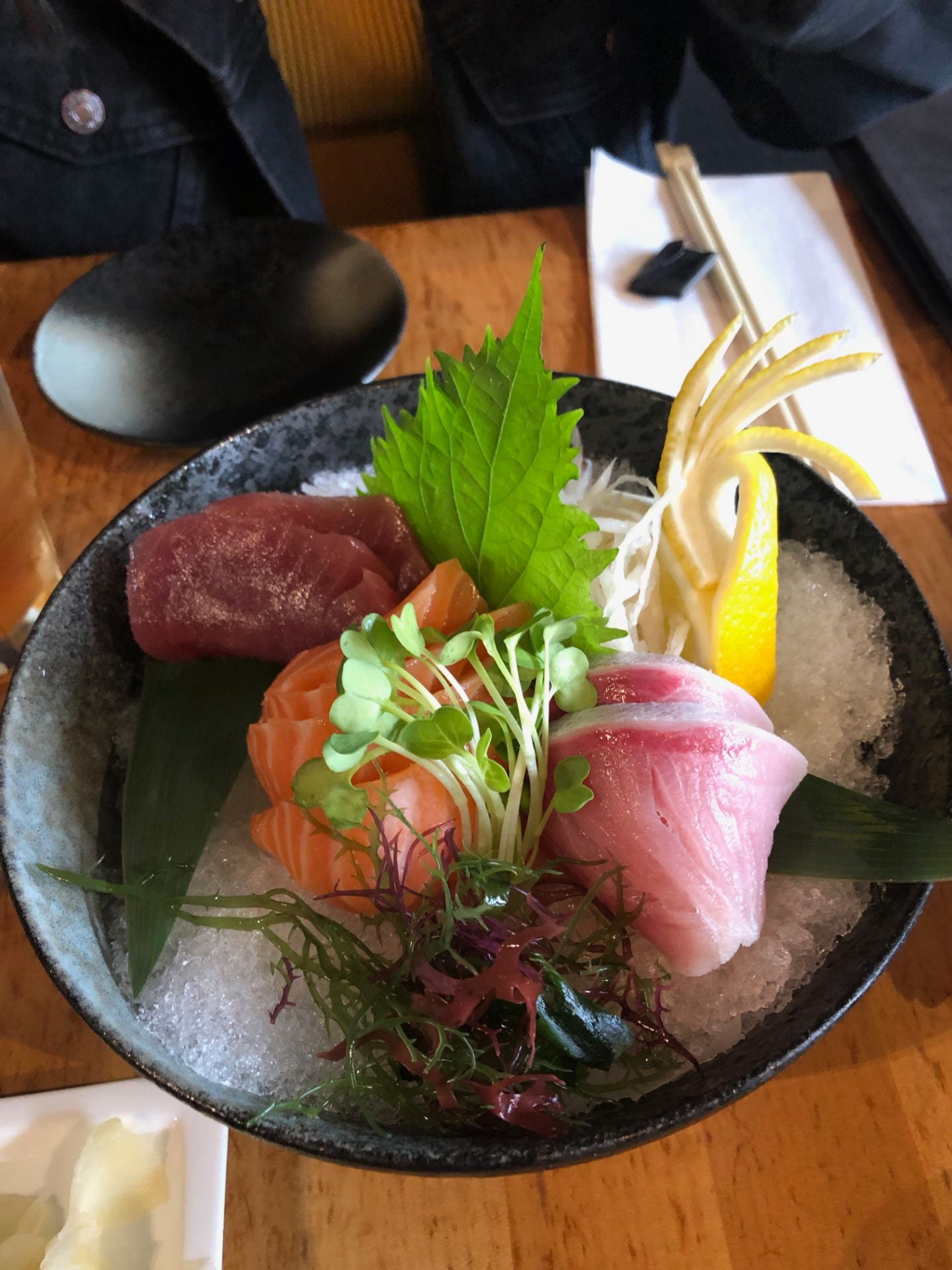
Location: Ginza Sushi & Bar

• The fish were stored in the freezer until lab on Tuesday, September 3rd.

 

Tuesday, September 3rd 2019

DNA Extraction From Animal Tissue Protocol

Reagents: Commercial DNA Extraction Lit (Sigma REDExtract-N-Amp Tissue PCR Kit)

• Extraction Solution (labeled ES)
• Tissue Preparation Solution (labeled TPS)
• Neutralizing Solution (labeled NS)

Materials:

• P200 microcentrifuge
• 5 mL microcentrifuge tubes
• Razor blades
• Heat block
• Vortex
• Ice
• Sharpie
• Gloves

1. Recorded the information about my samples on the “Animal Tissue DNA Extraction” data sheet along with giving each of my samples a unique ID code.

MM01 – Akami, MM02 – Salmon, MM03 – Yellowtail, MM04 – Maguro

2. Put on gloves and labeled one 1.5 mL screw-cap/lock lid microcentrifuge tube for each of my samples with the unique ID code. Used a sharpie to write the unique ID code on the side and on the top of each of the tubes.

3. Took my samples to free table to cut out a small piece.  Using a razor blade, I carefully cut out a small square of tissue on a paper plate.  Also made sure to clean the cutting utensil with Ethanol between specimens, and cut them on different parts of plate.

4. Weighed my sample on the scale using a weigh boat ( ~ 2 – 10 mg ) of sample tissue.

5. Added 100 mL of Extraction Solution (ES) to each of your labeled sample tubes using a p200 µL micropipette and filtered tips

6. Added 25 mL of Tissue Preparation Solution (TPS) to the microcentrifuge tubes with the 100 mL of Extraction Solution (ES) and micropipetted up and down to mix using a p200 µL micropipette and filtered tips.

7. Carefully added each sample to its corresponding extraction microcentrifuge tube using forceps.

8. Took a disposable non-filtered pipette tip and mashed my tissue sample up a bit.

9. Incubated the sample at room temperature for 10 minutes.

10. Moved my samples to the heat block and incubated the sample at 95^o C for 3 minutes.

11. Took the sample out of the heat block.  Added 100 ml of Neutralizing Solution (NS) using a p200 pipette and filtered tips and mixed by vortexing to vigorously mix up my samples.

12. Placed my samples on ice for the time being.

Amplifying CO1 from Fish  Procedure

To amplify COI from my fish DNA, I used components that came in the same kit that I used to isolate genomic DNA (gDNA). The Sigma REDExtract-N-Amp Kit included a solution for use in PCR amplification that includes Taq, dNTPs, and buffers that work optimally given the reagents that are still in your gDNA sample from the isolation procedure

USED FILTER TIPS FOR ALL PCR STEPS

Diluting gDNA 

10x dilution of my gDNA:

1. Labeled a microcentrifuge tube at my lab bench with “1:10”, the name of each my samples and initials on the top and side of the tube.

2. Added 18 mL of purified water to the labeled tubes.

3. Added 2 mL of my gDNA to the tube.

4. Gently flicked the tube to mix the solution.

PCR Reaction

Each of the PCR reactions included the following reagents and volumes:

Reagent                                                            Volume

Water (PCR Quality – autoclaved, filtered)     6.4 µl

REDExtract-N-Amp PCR rxn mix                  10 µl

Forward Primer FbcF                                       0.8 µl

Reverse Primer FbcR                                       0.8 µl

Tissue Extract (gDNA) (1:10 dilution)            2 µl

Total Volume                                                  20 µl

 

The standard procedure when setting up multiple PCR reactions under the same conditions is to make a master mix that includes the combined volumes of all of the reagents for multiple reactions, except for the component that is different. This improves success by minimizing errors due to pipetting small volumes multiple times.  For this reaction, I made up a master mix that included all reaction components except gDNA.  One master mix was made for my entire lab table.

The convention for making a master mix is to use the volumes for the individual reactions (listed above) multiplied by the number of reactions, plus some extra just in case.  For example, if we have 6 samples, one negative control, and we want to make sure we have a little extra.  So we would multiply the volumes times 6 + 1+ 1 = 8.

The additional reagents are needed to account for minor errors in pipetting that could result in not having enough total volume in the master mix for all individual reactions. A negative control is all the reagents required for a PCR reaction, but NO gDNA template.  Thus, if anything is amplified in the negative control, you know there is a source of contaminating gDNA, other than the samples you are trying to PRC amplify.

Master Mix Recipe:

Reagent                                                  Volume (1x)      Master (volume x 18)

Water (PCR Quality)                              6.4 µl                  115.2 µl

REDExtract-N-Amp PCR rx mix           10 µl                  180 µl

Forward Primer                                       0.8 µl                  14.4 µl

Reverse Primer                                        0.8 µl                 14.4 µl

Tissue Extract (gDNA- 1:10 dilution)    2 µl                     ———

Total Volume                                         20 µl                324 µl

 

1. Wrote the labels of my gDNA sample on my PCR tubes on the top and side below the lid.

2. Added 2 mL of the 1:10 dilution of my gDNA to each of the PCR tubes, except the negative control.  Made sure that my gDNA and mastermix were mixed together and changed tips between each sample.

3. Pipetted 18 mL of the master mix into each of my PCR tubes, including the negative control.

I left this reaction on ice next to the thermocycler until all PCR reactions were set up.  Then I placed the PCR tubes (all samples and the negative control) in the thermocycler and started the reaction, which took between 1.5-2 hours. MyPCR reactions will be placed in the freezer when the cycling is complete.

Settings for the Thermocycler:

94^o C – 4 min (initial denaturation)

30 cycles of:

94^o C for 30 sec (denaturing)

52^o C for 40 sec (annealing)

72^o C for 1 min (extension)

72^o C for 10 min (final extension)

10^o C hold

Fish DNA Barcode

Tuesday, September 17, 2019

Gel Electrophoresis/PCR Cleanup

Gel Electrophoresis of PCR products:

1. Grabbed PCR tubes from ice and thawed
2. Dotted out 16 loading dye dots (1 µL) on a sheet of parafilm
3. Pipetted 3 µL of each PCR product into its own dot
4. Loaded all the dots into the gel (5 µL each)
5. Ran the gel at 130 volt for 30 minutes

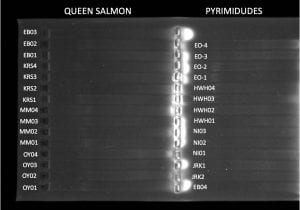
Gel Electrophoresis Loading Order for Queen Salmon:

Lane #   Sample ID #

TOP

1                OY01

2               OY02

3               OY03

4               OY04

5               MM01

6              MM02

7              MM03

8             MM04

9             KRS 01

10           KRS02

11            KRS03

12           KRS04

13           Negative Control

14           EB01

15           Ladder

BOTTOM

16           EB02

17           EB03

18          EB04

19          Ladder

Clean-up of PCR products for sequencing – ExoSAP:

1. Labeled new 0.2 µL PCR tubes with each of my sample codes (MM01, MM02, MM03, MM04) and shared an 8-strip with my lab partner which will be sent off for sequencing.
2. Determined the number of PCR clean-ups my table will make up.
3. Calculated the volume of Master mix needed (calculated for a couple additional cleanups to account for pipette errors).
4. Placed reagents on ice.
5. Pipetted 7.5 uL of each PCR product into a clean, labeled 0.2 uL PCR tube.
6. Made up the ExoSap master mix, keeping the reagents on ice while it was made.
7. Pipetted 12.5 uL into each PCR product tube.
8. Placed the tubes in a thermocycler and started the EXOSAP program.
9. After program completed (~ 45 minutes) placed PCR tubes in a labeled tube rack and put in the freezer.

ExoSap PCR Clean-Up Protocol

Recipe to clean-up one PCR reaction of 7.5 uL

Master Mix:                                 Rxn: 1                Rxns: 18

H₂O                                               10.59 uL            190.6 µL

10x buffer (Sap 10x)                   1.25 uL              22.5 µL

SAP                                               0.44 uL              7.92 µL

Exo                                                0.22 uL              3.96 µL

Master Mix Total                       12.5 uL              225 µL

PCR Product:

PCR                                               7.5 ul

Total Cleaned-up Volume        20.0 uL

 

Tuesday, October 1st 2019

Geneious Lab (DNA and protein sequence data)

*Followed protocol*

• Created a folder to store my fish barcodes and downloaded the classes DNA barcoding sequences (forward and reverse reads) from Canvas which were dropped into my fish barcode folder
• My PCR failed completely because the sequence was very short.  Therefore, I had the DNA sequences of another students from a previous year (KJ01 and KJ02)
• At the sequence view, reverse complimented my sequence so that the orientation was switched and the base call were complimentary to the previous one.
• Assembled forward and reverse sequence reads of the same sample —- copied the reverse sequences from the ‘Fish barcode Reverse Reads’ folder and pasted them in the ‘Forward Reads’ folder.  Selected two of my sequences that have the same ID but one was indicative of forward and the other of reverse.  Right clicked and chose ‘De novo assembly.’
• Clicked ‘Allow Editing’ and deleted any bases on the two ends that were unreadable  — this is important because it only keeps the base calls that I have confidence in.
• Looked at the consensus sequence for any ambiguities (N, Y, R) and determined its discrepancy; edited the sequence with the poor read to match the base call of the good read.
• Closed and saved my sequence assembly.
• Selected the assembly file that I just saved and right clicked ‘Generat consenseus sequence’ and kept the default settings.
• Selected the new consensus sequence file and right clicked ‘BLAST’ that will search the database for highly similar sequences
• Hit Table opened up a  set of the 100 top matches to my sequence.
• Built an alignment with my sequence and some of the top 100 hits
• Created a new folder ‘Fish barcode test alignment’, went back to my fish barcode colder and selected ‘…assembly consensus sequence’ file, right clicked and chose ‘Copy documnet’ and selected the new ‘Fish barcode test alignment’ folder to paste it in.
• Scrolled through BLAST search results and selected about 5-10 hits and copied it into the ‘Fish barcode alignmnet’ tab.
• Double clicked the ‘nucleotide alignment file’ to open the alignment and noticed any polymorphisms in my alignment (looked at the consensus identity for the ambiguity code)

1.  The sequences for the species sampled (KJ01) stated it was a Thunnus albacares (yellowfin tuna) which was the same type of fish that the student thought their fish to be.  The sequences for the species sampled (KJ02) stated that it was a Oncorhynchus tshantytscha voucher (chinook salmon) otherwise known as king salmon which was the same type of fish that the student thought their fish to be.
2. First 10 polymorphic sites found in the alignment based on the column found for KJ01 (4 sites) and KJ02 (13 sites)

KJ01

• Column 9 – [C] consensus identity: GU673630
• Column 21 – [T] consensus identity: GU672630
• Column 42 – [A] consensus identity: GU324196
• Column 273 – [T] consensus identity: GU673630

KJ02

• Column 55 – [G] consensus identity: JX960909; [C] consensus identity: FJ998625; [A] consensus identity: FJ998949
• Column 69 – [A] consensus identity: FJ998625
• Column 78 – [G] consensus identity: FJ998625
• Column 108 – [T] consensus identity: FJ998625
• Column 113 – [T] consensus identity: FJ998625
• Column 117 – [C] consensus identity: FJ998625
• Column 123 – [A] consensus identity: FJ998625
• Column 165 – [C] consensus identity: FJ998625
• Column 171 – [A] consensus identity: JX960909; [A] consensus identity: FJ998625
• Column 204 – [C] consensus identity: FJ998625

Consensus sequence of KJ01, KJ02, and 25 sequences of the COI gene from Actinopterygii

-included one ray (outgroup)

Tuesday, October 8th 2019

Geneious Lab (Phylogenetic Inference)

• Cleaned up my alignment of COI sequences (fish DNA barcode sequences and sequences downloaded from NCBI through Geneious) by editing the alignment down so that all sequences begin and end at the same point — clicked ‘Allow Editing’ and chose the bases (all the columns in the alignment) that precede where the sequences start (blue selected parts) and the ones that are beyond the sequences (blue selected parts)
• Looking at my sequence, I found 9 columns of my alignment to be polymorphic \

Choosing the best model of Molecular Evolution:

• Used the jModelTest2 program (downloaded) to figure out the best model of molecular evolution for my sequences.
• Exported my alignment in Geneious in Phylip format (relaxed) – selected my alignment and from the top ‘File’ menu chose ‘Export > Selected documents >’ and once a new window appeared, scrolled down to ‘Phylip(*.phy)’ and clicked ok.  A window appeared after I chose where to save the file and selected the ‘releaxed’ format.
• Went back to the jMOdelTest2 program and opened the exported alignment using ‘File > Load DNA Alignment’ in the menu.
• Selected ‘Analysis > Compute likelihood scores’ from the menu.  Kept the defaults that are in the next window and chose ‘Compute Likelihoods.’  The program took about 10-20 minutes because it went through a hierarchal set of 88 models (increasing complexity) and calculated the likelihood for each of those models of molecular evolution, based on an initial tree that is used for all tests.
• Two methods are used: Akaike Information Criterion (AIC) and Bayesian Information Criterion (BIC).  Under the Analysis menu chose ‘Do AIC,’ a window appeared, kept the defaults, and clicked ‘Do AIC calculations.’  This analysis is done instantaneously.   In the main jModelTest window clicked ‘Results > Show results table’ and clicked the ‘AIC’ tab at the top.  Clicked on the ‘AIC’ column to bring the top scoring model to the top (red).  My best model based on AIC is: GTR + I + G
• Followed the same steps from above to check the best model based on BIC.  My best model based on BIC: GTR + I + G.  The AIC and BIC chose the same model.  The comparison of these models are important because more complicated models will always have a better fit, but it is necessary to see if the better fit is worth the cost of the extra parameters.

Bayesian Inference

• Selected my alignment in Geneious, right clicked to select “Tree…” and chose ‘MrBayes.’  Chose the ‘GTR’ (complicated) substitution model — closest to the jModelTest choice in complexity.
• Looked at the ‘Rate Variation’ and chose ‘I + G( (invgamma).’  Chose the Chondrostroma voucher as my outgroup.  Looked under the MCMC settings.  The ‘Chain length’ is how many samples of the posterior distribution my analysis will use.  In a real analysis this number will be very large (10-50 million).  Set it to 10,100.  My ‘sample frequency’ is how often I actually save the inferred trees for the posterior distribution – don’t want this to be too small (less than 100) because I may sample trees with only very slight differences.  It’s better to sample a little bit more sparsely — used the default of 200.  Below ‘Subsampling freq’ there is ‘Burn-in length.’  This is the # of samples that should be removed at the beginning of my analysis because MCMC is a ‘hill-climbing’ algorithm indicating that the samples from the beginning are probably poor estimates of the phylogeny.  This set to 100.
• The number of trees sampled will be the number of samples (10,100) – the burn in (100) = 50.  The heated chains remain at 4 and the heated chain temp and random seed defaults remain the same.
• Priors used: ‘Unconstrained Branch Length: Exponential (10), Shape Parameter (10) — these affect the shape of the prior statistical distribution.
• Ran my analysis.  Double clicked the ‘Posterior Output’ line which opened a new window.  Clicked the ‘Parameter estimates tab.’  Clicked on the ‘Trace’ tab which showed an upward slope (increase in posterior probability).  The analysis was too short and did not do a good job sampling the posterior distribution.
• Clicked the ‘Tree’ tab to look at the inferred tree.  Clicked ‘Show Branch Labels’ and for ‘Display’ chose posterior probability.  This labels the branches with their support values based on the percentage of the trees that had a particular clade present.
• Ran the analysis again but used 100,000 for the ‘chain length’ and 10 for the ‘burn in.’  I recovered the same clades in my tree but they didn’t have the same similar support values.

Maximum Likelihood

• Used maximum likelihood to infer a phylogenetic tree of my aligned data set.  Installed the plugin RAxML.
• Chose my evolutionary model (similar choices to the Bayesian analysis) and chose ‘Rapid bootstrap with rapid hill climbing.’
• When RAxML is done, there is a new line called ‘RAxML bootstrapping trees.’  To build a consensus tree, selected this line, right clicked ‘Tree’ ‘Consensus Tree Builder,’ ‘Create consensus tree,’ and ‘Support threshold’ of 50% and ok.  The consensus tree will be listed as the 1st tree in the ‘RAxML bootstrapping trees’ file.  The clades with higher support don’t match those from my Bayesian analyses.
• Downloaded the PHYML plugin and ran a maximum likelihood with bootstrapping in PHYML.  Used the HKY85 model of molecular evolution for this and the final Bayesian tree.  Used the tree window to manipulate the resulting best ML tree with bootstrap support.  Made a ray species the root, showed the bootstrap proportions, and made the tree aesthetically pleasing by adjusting the line weights, font size, and tree display.
• Ran the same alignment and the HYY85 model of molecular evolution to infer my best tree using MrBayes.  This was ran at 3,000,000 generations, subsample frequency set to 500, and set my burn-in 300,000.  Chose the ray species as the outgroup.  When the run is complete, the final tree with support values, posterior distribution, and the trace was exported.

 

Welcome to your brand new blog at University of San Francisco Sites.

To get started, simply log in, edit or delete this post and check out all the other options available to you.

For assistance, visit our comprehensive support site, check out our Edublogs User Guide guide or stop by The Edublogs Forums to chat with other edubloggers.

You can also subscribe to our brilliant free publication, The Edublogger, which is jammed with helpful tips, ideas and more.